ADS1282 spectral noise floor

Yes and figures 7 through 10.

Thank you,

Frank

Frank, 

Figure 7,8 is data taken with inputs shorted. You can see the small idle tone components near DC.

Figure 9,10 is data taken with 20mV offset. The offset voltage moves the idle tones out of the passband, so no idle tones are visible.

The plots are simply FFTs of the conversion data. The condition for the data is listed in the graph and at the top of the page.

I received further clarification on the question.

Background: in order to use this part in our design, I modeled its function to simulate and predict certain performances. However, my model was not consistent at recreating information in the data sheet UNLESS I made certain assumptions regarding the methodology of generating the Output Spectral Plots.

How EXACTLY are the Output Spectrum Plots, as shown in Figures 1-6 on page 7 of ADS1282 data sheet, generated?

Thank you,

Hello Frank,

I am not sure if this is the information the customer is looking for, but this is a description of the test set up used to generate the curves on the datasheet

AVDD, AVSS=+/-2.5V
fclk = 4.096MHz using a crystal oscillator
fdata=1000SPS (Sinc+LPF)
VREFP+2.5V, VREFN=-2.5V (REF5050+OPA277 on EVM)

The 31.25Hz signal was generated using an Audio Precision Signal Generator SYS-2722; with a fully differential amplifier OPA1632; connected as shown on the ADS1282EVM.

The 8192 point FFT plots were generated using Low Sidelobe window function.

Please let me know if any additional information is required.

Thank you,

Luis

From your description, you have verified that the 31.25 Hz is not synchronized to the ADC at all.

What are the EXACT coefficients used in the "Low Sidelobe Window" function? Can you locate the exact weighting function used to create the curves in the data sheet?

BACKGROUND: To prevent excessive sidelobe generation from an FFT of an asynchronous pure tone signal, a weighting window is applied to the data before the FFT is calculated. In this case the window function consists of 8192 coefficients that are multiplied times the 8192 data points with the products used to calculate the FFT. Shape of the window function greatly impacts the results. Two, often used weighting functions, are hamming window and hanning window. Hanning [to me] is preferable. The hanning window is similar to the well-knwon hamming window. It is also an offset single cosine window. However, with the hanning window the weighting function starts at zero, goes to a peak in the center of 2, and back down to zero following the cosine curve. The peak of 2 is used to keep the average signal information normalized, maintaining proper amplitude of the resulting FFT.

I will review the EVK and its use of the OPA1632.

Thank you,

Frank

Hello Frank,

The differential amplifier (OPA1632) on the ADS1282EVM set up is mainly used to keep the common mode voltage constant.  This is in order to not have common -mode rejection errors on the measurements.  Since the ADS1282 device already has a built in PGA to drive the Delta-Digma modulator, the primary function is only to set the common mode voltage when the Audio Precision signal generator is connected to the device.    

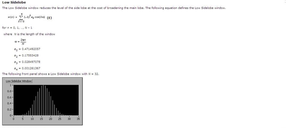
The FFT 8192 point FFT plots where generated using the "Low-Sidelobe" FFT Window function built into the Lab View software package.  The Low Sidelobe function was chosen since it provides the best rejection at the side lobe at the cost of broadening the main lobe.  This window function is similar to the Blackman-Harris.

Below is a section from the Lab View help file that shows some of the coefficients of the Low Sidelobe function.  I noticed that "a1" coefficient is missing on the description and I suspect this is a typo on the help file.  Attached is also a PDF file with the complete Lab View help  regarding the "Characteristics of Different Smoothing Windows" in the Lab View help menu. 

I hope this helps. 

Regards,

Luis

1050.LV_Window_Help_file.pdf