

Other Parts Discussed in Thread: DRV5055, , TMAG5273
A major benefit of using a Hall-effect sensor in position sense applications is that it eliminates the physical contact needed to determine position in mechanical solutions. This occurs due to the permeation of magnetic flux from a nearby magnet, which can be used by a linear Hall-effect sensor to produce an output that varies with the changing input field. The magnetic field permeates through air, dust and grime, plastics, and other generally non-ferromagnetic materials. As a result, the sensor can be conveniently placed anywhere a measurable magnetic field is present to provide feedback. One particular challenge that is present when using a linear output Hall-effect sensor is that the magnetic flux density is inversely proportional to the square of the distance from the magnet. As a result, this adds some complexity to position calculations as linear steps produce a non-linear change on the output. While this can be calibrated for any particular magnet, one useful configuration is to orient the magnet and sensor in a slide-by configuration. Here, instead of traveling directly towards the sensor, the magnet travels just above the sensor in a linear path.
As an example, consider the arrangement of a one-dimensional sensor, such as DRV5055 shown in Figure 1 with the magnet traveling either direction along the black line which is parallel to the Y axis. In this example, the pictured magnet is about 22 mm thick with a radius of about 3 mm.
FIGURE1 - Slide-By Magnet Orientation
In this configuration, the sensor will only detect the component of the field vector which is directed along the Z-axis. The resulting input to the sensor over the course of travel for this magnet has an interesting behavior. There is a region approximately the same length of the magnet which produces a linear change in field. With this input, it is now simpler to monitor change in position by measuring in the linear input region.

FIGURE2 - Slide-By Input Field
This can also be easily adapted to increase overall stroke length through the addition of multiple sensors. The process involved with this type of design is discussed in greater detail in Linear Hall Effect Sensor Array Design.
The one dimensional case is limited in range by the length of the magnet. Travel outside the linear input region produces uncertainty in position as there are now two positions that map to the same input magnitude. The uncertainty is resolved by using a three dimensional, 3D, sensor instead. With this sensor type an input field shown in Figure 3 can be observed.
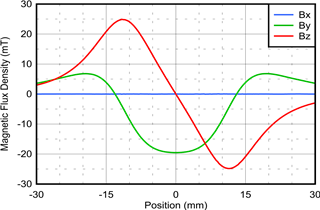
FIGURE3 - 3D Slide-By Input Field
Using this input, three distinct input regions can be defined. The linear region still provides the best correlation for linear motion, but based on the Y component, it is now possible to distinguish the direction approach of the magnet in the non-linear regions as well. Suppose a -6 mT limit is set for By to correspond to the peak values of Bz.
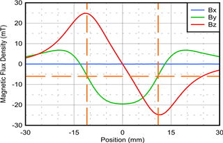
FIGURE4 - Input Field Regions
When By exceeds this threshold the magnet is known to be in the linear sensing region. For By below the threshold, then the sign of Bz will indicate whether the approach is from the right or left. Calibrations can be used to determine the position in this non-linear region, and accuracy will diminish as the magnet moves further from the sensor.
A similar and advantageous approach will again utilize a 3D sensor, but this time the magnet pole will be directed normal to the sensor face rather than parallel. The magnetic field profile across the magnet travel is very similar to the previous example.
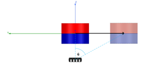
FIGURE5 - Slide-By Mechanical Angle
As the magnet is moved along the Y axis, this motion will produce inputs as shown in Figure 6. In this case, the magnet is much smaller than before with an approximate thickness of 5 mm and a radius of 3 mm. As a result of the orientation change of the magnet, the linear region is now observed on the By component. The width of this region for this particular case is only 6 mm.
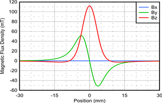
FIGURE6 - Angle Measurement Inputs
Using this data, it is would be possible to use only By to track position, but using the arctangent function will enable position detection over a much wider range.
Electrical Angle: θ = atan 2( Bz , By) 1
Comparing the calculated electrical angle based on the magnetic field inputs to the actual mechanical angle between the magnet and sensor reveals an interesting behavior.
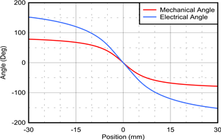
FIGURE7 - Measured Angle vs. Position
While there is a significant error between these two calculations as a result of using magnetic field inputs which do not strictly follow a sinusoidal behavior, it is apparent that the general form of the electrical angle calculation follows the behavior of the mechanical angle. Given this similarity, it should be possible to adjust the electrical calculation to match the actual mechanical angle. When using TMAG5170, it is possible to apply both a gain and offset correction to a single channel which can be represented as α and δ, respectively. Additionally, it is apparent that a second scalar would be beneficial to decrease the overall magnitude. This scalar will be represented by β. This correction would be applied by a microcontroller which is recording the outputs of TMAG5170. Closer analysis also shows that a scaling factor, γ, that increases with angle, can also be helpful in aligning the asymptotic behavior of the two curves at the furthest magnet positions. An example equation based alignment with each of these factors is shown in Equation 2 and Equation 3.
θ′ = atan2 (α × (Bz + δ) , By) 2
θ = β × θ′ − γ × sin θ′ 3
To enable demonstration of this function, please consider the attachment for TMAG5170 EVM shown in Figure 8. Files to enable 3D printing this attachment and physical geometry are available in TMAG5170 Slide-By Attachment.
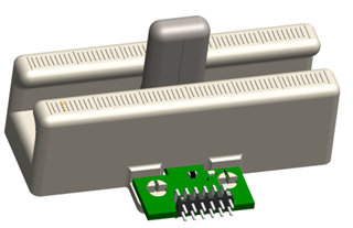
FIGURE8 - TMAG5170 Slide-By Attachment
Based on the simulation data and results of Equation 2 and Equation 3, there are multiple possible implementations with their resulting accuracies. These values and respective errors were determined through inspection. Other methods of linearization, including multipoint calibration, can also prove successful approaches to linearize results. In the following examples three configurations are shown. Configuration 1 applies a scalar correction to the Z axis, and then scales the magnitude of the resulting angle output. Configuration 2, uses these factors as well, but includes an additional intentional offset to help expand the sensitivity range. To help limit error further, configuration 3 adds the final correction factor to help further extend the viewable range of the sensor to the point where input referred noise will likely become the predominant factor for position accuracy.
Table 1. Configurations and Measurement Ranges
|
Configuration |
α | β | δ | γ | Range | Accuracy |
| 1 | 0.6075 | 0.786 | 0 | 0 | +/- 11mm | +/- 0.06mm |
| 2 | 0.6145 | 0.795 | 0.43 | 0 | +/- 21mm | +/- 0.25mm |
| 3 | 0.534 | 0.87 | 0.24 | -7.25 | +/- 23mm | +/- 0.1mm |
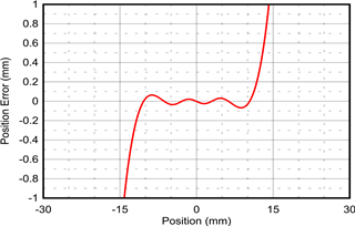
FIGURE9 - Configuration 1
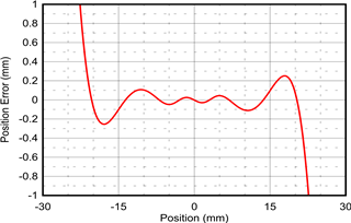
FIGURE10 - Configuration 2
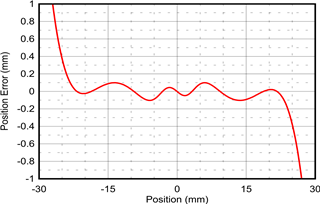
FIGURE11 - Configuration 3
It is also important to remember that these results can vary from system to system as sensitivity error, offset, noise, and mechanical variations will all impact these results which are the theoretical best case behavior. Additional calibration factors can be implemented to improve overall accuracy.
Table 2. Alternative Device Recommendations
| Device | Characteristics | Design Considerations |
| DRV5055 (DRV5055-Q1) | Commercial (Automotive) single axis bipolar linear Halleffect sensor with Analog output available in SOT-23 and TO-92 packages | Analog outputs are subject to electrical noise and calculations require MCU computations. Single axis sensitivity constrains the ability to track movement in free space. |
| DRV5057 (DRV5057-Q1) | Commercial (Automotive) single axis bipolar linear Halleffect sensor with PWM output available in SOT-23 and TO-92 packages | PWM outputs require conversion, but are less susceptible to coupled noise. Single axis sensitivity constrains the ability to track movement in free space. |
| TMAG5170 (TMAG5170-Q1) | Commercial (Automotive) grade linear 3D Hall-effect position sensor with SPI interface available in 8 pin DGK package | Complete magnetic vector sensitivity. This device is able to track a wide range of magnet positions, though careful planning is still required to ensure all input conditions map to a unique position. |
| TMAG5273 | Linear 3D Hall-effect position sensor with I2C interface available in 6 pin SOT-23 package | TMAG5170 has a tighter sensitivity tolerance and TMAG5273 operates over I2C |
Table 3. Related Technical Resources
| Name | Description |
| Linear Hall Effect Sensor Array Design | A guide to designing sensor arrays for tracking motion across long paths |
| Intro to linear Hall effect sensors: Achieve contactless accurate position sensing | A discussion on the differences between a linear output and switched output Hall-effect sensors. |
| What is a Hall-effect sensor? | A discussion about the Hall-effect and how it is used to create magnetic sensors |
| TMAG5170UEVM | GUI and attachments incorporate angle measurement using a precise three dimensional linear Hall-effect sensor |
| TMAG5273EVM | GUI and attachments incorporate angle measurement using a three dimensional linear Hall-effect sensor |
| DRV5055EVM EVM | EVM incorporates a digital display with various sensitivities aligned linearly along a ruler face. |
| TI Precision Labs - Magnetic Sensors | A helpful video series describing the Hall effect and how it is used in various applications |
Source: www.ti.com/.../sbaa513.pdf