

If you have a voltage divider where each resistor has 5 ppm/°C drift, what is the worst-case drift? That is the loaded question I posed to my colleagues recently (only after figuring out the answer myself, of course) while working on a low-drift current sensing reference design (TIPD156). The ‘obvious’ answer is 10 ppm/°C. It turns out to be just 5 ppm/°C, but only when the voltage divider ratio is ½. Let us delve deeper into the answer to this obvious, yet not-so-obvious question.
Figure 1 depicts a discrete solution that provides a reference voltage (VREF) and bias voltage (VBIAS) based on the ratio of R1 and R2.

Figure 1: Dual reference discrete topology
At the time it was ‘obvious’ that the overall drift of the resistor divider is (5 ppm/°C) + (5 ppm/°C) = 10 ppm/°C. Just to be sure, though, I ran a simulation. Figure 2 depicts the result of the TINA-TI simulation where R2 drifts in the positive direction, R1 drifts negatively, and the change in temperature is 100°C.

Figure 2: Vbias after R1 and R2 drift
Calculating the gain error yields 0.05% (500 ppm or 5.0 ppm/°C), which is the drift of one resistor…not their sum!
Now let’s examine the familiar voltage divider circuit’s gain ratio and re-arrange it as shown in Equation ( 1 ).


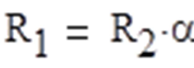
α is the ratio of R1 and R2, and ultimately relates to the gain of the circuit. For example, if α=1, the gain is ½. So, as α→0, the gain→1. Similarly, as α→∞, gain→ 0.
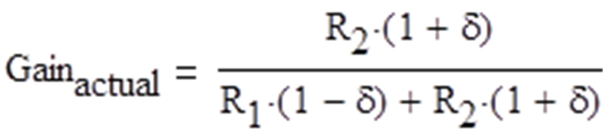
The actual gain of the circuit over temperature will depend on the drift of the resistors, which is shown in Equation ( 3 ) by δ. To be consistent with the simulation, R2 drifts positively and R1 negatively.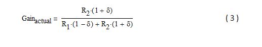
Equation ( 4 ) calculates the gain error. For simplicity, it is not converted to a percentage (if you want to do that, simply multiply it by 100 but be careful when converting to ppm).
 Using Equations ( 1 ) to ( 3 ), Equation ( 4 ) simplifies to:

Notice that the gain error depends on both the drift (δ) and the circuit gain (related to α). Furthermore, if α=1 (circuit gain=½), the gain error simplifies to δ, which is exactly what the simulation shows!
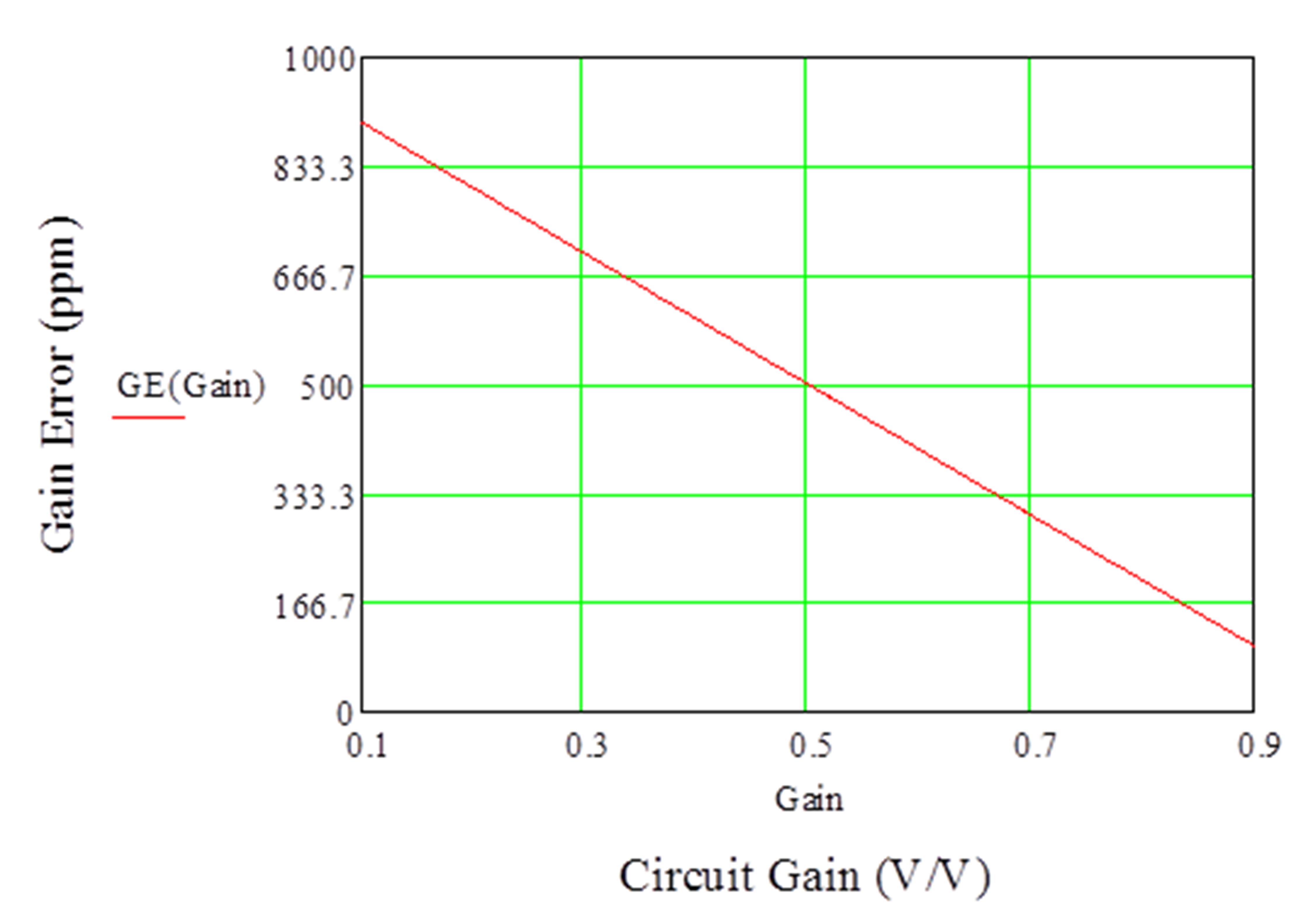
Figure 3 is a plot of the gain error versus the circuit gain for this design (5 ppm/°C resistor drift, or 500 ppm total drift over 100°C). Notice that the gain error is 500 ppm when the circuit gain is ½. Also notice that as the circuit gain increases, the gain error decreases and vice versa.
In summary, the drift of the voltage divider was not as expected…it is not the simple sum and it depends on the circuit gain. So, next time you’re designing a circuit and come across one of those ‘obvious’ conclusions, you may want to double-check it with TINA-TI!
If you have any similar ‘obvious’ experiences, please share them in the comments section!
-

Chris Belting
-
Cancel
-
Vote Up
0
Vote Down
-
-
Sign in to reply
-
More
-
Cancel
Comment-

Chris Belting
-
Cancel
-
Vote Up
0
Vote Down
-
-
Sign in to reply
-
More
-
Cancel
Children