This thread has been locked.

If you have a related question, please click the "Ask a related question" button in the top right corner. The newly created question will be automatically linked to this question.

IWR1443BOOST: reading raw data from DC1000EVM

Part Number: IWR1443BOOST
Other Parts Discussed in Thread: DCA1000EVM, AWR1642BOOST, AWR1642, IWR1642, IWR1443

Dear experts,

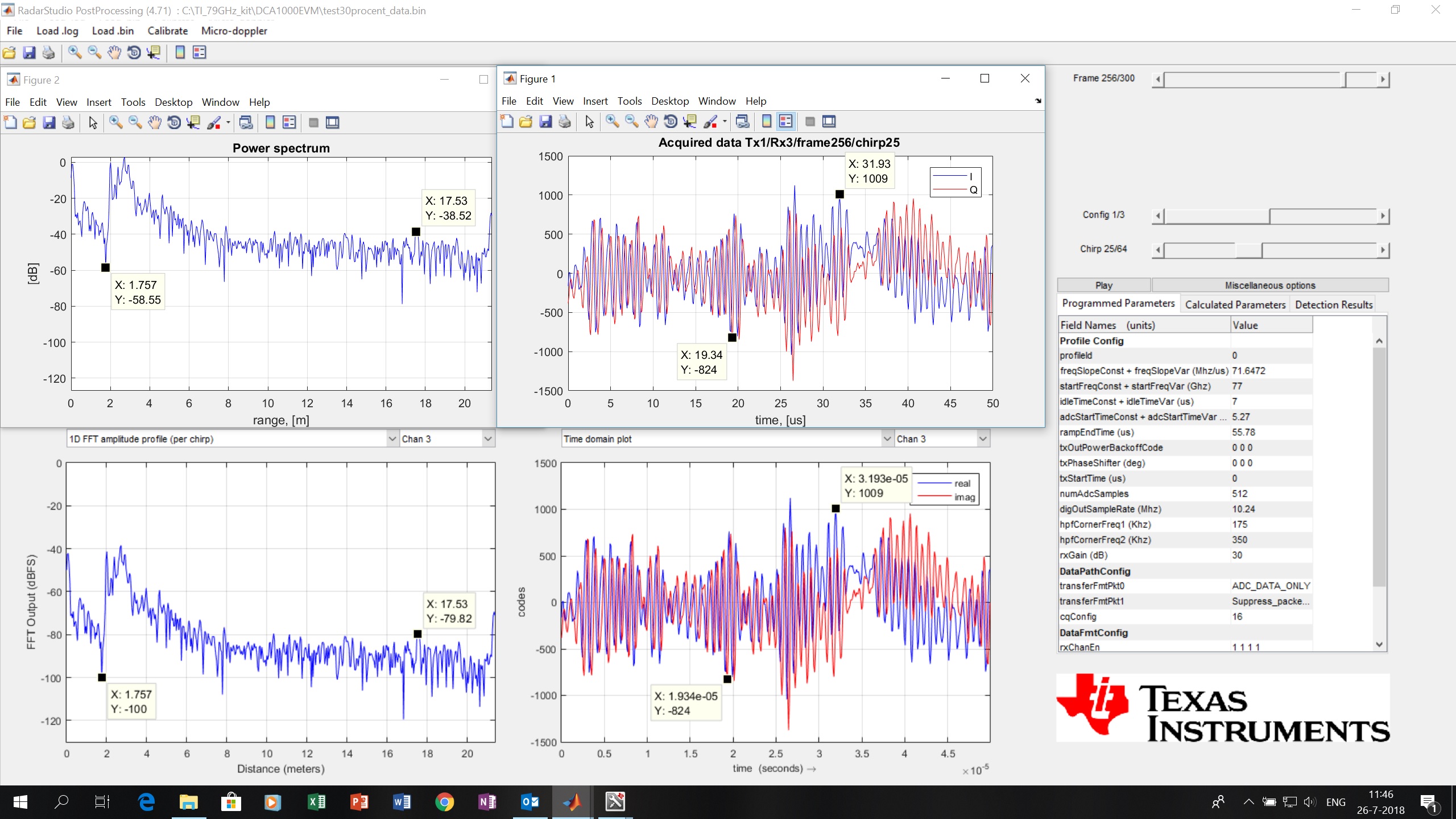
my setup IWR1443Boost+DC1000EVM is up and running, now I can do long acquisiitons with infinite number of frames by simply pressing START and STOP buttons in mm-Wave Studio. Could you provide a MATLAB script that reads and parses raw data correctly? I see the data format has changed, and on top of that the UDP packets might be missing sometimes so it would be very helpful if you share a script-example to read the data. The data post-processing implemented in mm-Wave Studio at first corrects for missing packets, creates file "adc_data.bin" from "adc_data_Raw_0.bin", and then delivers a MATLAB Figure with plots. I need a script which allows me to do the same in MATLAB for a flexible number of  "adc_data_Raw_N.bin". 

Thanks and regards,

Timofey

  • Hi Tomofey,

    Sorry it's beyond of current support.

    Regards,
    Michelle
  • Hello Michelle,

    pity! Then could you explain more on the raw data format? My meaurement parameters:
    - 3 Tx / 4 Rx;
    - complex 1;
    - 512 samples per chirp;
    - 64 chirps per frame;
    - 300 frames.

    I assume this is case 22.6 in mmWave Studio User's Guide, p. 57 but even that description looks unclear. The second row shows sample 4 after sample 0 in the first row. What happened to samples 1-3 then?
    Thank you very much in advance.

    Best regards,
    Timofey
  • Hi Timofey,

    I think you are right, the 2nd row should be the 2nd sample for rx0 to rx3.
    I'll report this issue in the document.

    Thanks and Regards,
    Michelle
  • Hi Michelle,

    I already tried to read the samples that way (0,1,2,3,4,..Ns-1) but it did not help much. The parsed signals look weird in MATLAB while they are good in mmWave Studio for the same dataset. If you provide a clear description of the new data format for my configuration I will highlight a few more critical issues that I solved to arrive at consistent data acquisitions with DCA1000EVM.

    I am trying to import the data based on my experience with TSW1400 accounting for the new order of samples in rx0-rx3. For TSW1400, my data reading procedure is given below:

    fid = fopen('adc_data.bin','r');
    N_data = Ns*N_chirps*N_rx*N_tx*2*N_frames;
    dat = fread(fid,N_data,'uint16');
    fclose(fid);
    dat = dat - 2^15;
    cdat = zeros(Ns,N_rx,N_tx,N_chirps,N_frames);
    sI = zeros(Ns,1);
    sQ = zeros(Ns,1);
    sIQ = zeros(Ns,1);
    k1 = 1;
    k2 = 8;
    k3 = 7;
    for kframes = 1 : N_frames
    for kchirps = 1 : N_chirps
    for ktx = 1 : N_tx
    for ks = 1 : Ns
    sIQ = dat(k1:k2);
    sIQ = reshape(sIQ,[2 N_rx]);
    sI = sIQ(1,:).';
    sQ = sIQ(2,:).';
    cdat(ks,:,ktx,kchirps,kframes) = sI + 1i*sQ;
    k1 = k2 + 1;
    k2 = k1 + k3;
    end
    end
    end
    end

    It takes 8 real samples, creates an IQ signal of 4 samples, and assigns those complex samples to rx0..rx3. Then next 8 samples... Then next transmitter... Then next chirp... Then next frame... This works fine and gives me the same waveforms as in Radar Studio. What changed exactly for DCA1000EVM and mmWave Studio?

    I also noticed that a raw data file "adc_data_Raw_0.bin" is always slightly larger than its post-processed in mmWave Studio version "adc_data.bin". The size of the latter corresponds precisely to N_data = Ns*N_chirps*N_rx*N_tx*2*N_frames. Unfortunately my procedure does not read both files correctly. I presume the post-processing in mmWave Studio removes a header and corrects for possibly missing UDP packets in "adc_data_Raw_0.bin".

    Hopefully this lets find a solution quickly, otherwise why we need DCA1000EVM if there is no way to read and process the raw data independently of mmWave Studio. Thanks a lot in advance!

    Regards,
    Timofey
  • I see your point. However, our support is limited to mmwave studio related only. Having said that, I still try to provide as much help as possible. Here's the table which may help you figure out the difference between DCA1000 and TSW1400:

    1. FPGA sends data in the following Ethernet packet format.

    Destination MAC

    (6 bytes)

    Source MAC

    (6 bytes)

    Type

    (2 bytes)

    Payload

    (46 - 1500 bytes)

    IPv4 header

    (20 bytes)

    Payload

    (Max - 1480 bytes)

    UDP header

    (8 bytes)

    Payload

    (Max - 1472 bytes)


    Sequence number

    (4 bytes)

    Byte count

    (6 bytes)

    Data

    (Min – 48 bytes

    Max – 1468 bytes)


  • Thank you Michelle. In return I would recommend to mention in User's Guide about Windows Defender Firewall which should allow the UDP to come through. This can be done in properties of mmWave Studio in Inbound Rules, Advanced Settings.
    What's happening next after FPGA sends data in the above packet format? How does mmWave Studio order frames/chirps/tx/rx/samples in the saved data?
  • Thanks for the suggestions. I wasn't aware we have the setting of firewall in mmwave studio. Can you let me know where I can get to the Inbound Rules, advanced settings?

    Thanks!

    Regards,
    Michelle
  • OK. When you look into Control Panel\System and Security\Windows Defender Firewall\Advanced settings you'll find Inbound Rules wherein you can define access properties (TCP/IP, UDP) for every installed application including mmWave Studio. Please consider working outside that Studio...

    BR
    Timofey
  • Timofey,

    Thanks. We will take your suggestions into consideration.

    Regards,
    Michelle
  • Hi Michelle,

    Tim's question about what has changed in the data format between the TSW1400 and the DCA1000 boards is still unanswered. The Radar Studio user's guide lists 2 formats for DCA1000, one interleaved and one non-interleaved. How does one know which format is applied? There is no further reference to interleaving in the whole user's guide.

    Thank you,
    François.

  • Francois,

    The interleaved and non-interleaved depends on the type of radar device. For xWR12xx/xWR14xx, only interleaved mode is supported. For xWR16xx, only non-interleaved mode is supported. See 22.6 to 22.9 of mmwave studio user guide.

    Let me know if you have any question.

    Thanks and Regards,

    Michelle

  • Hi Michelle,

    Thank you. I had not noticed the answer was indeed in the document's sections names.

    One more question: the Packet reorder and zero fill utility processes one 1 GB file at a time. What happens if some UDP packets need to be reordered across 2 consecutive files, as the utility sees one file at once?


    Thanks,
    François.
  • I'm not sure how that is handled across files. I've sent the question to our expert and will get back to you.
    Regards,
    Michelle
  • Hi Timofey,

    I have the same issue as you. Actually, I want to process the adc_data.bin file generated from the DCA1000EVM (DCA1000 + AWR1642BOOST). In the documentation, I only found a Matlab code used with TSW1400 but not for raw data generated from DCA1000.
    I am seeing the data analyzed in the PostProc module and also want to do the same (extract signals, frames..... etc ).
    Does the code also works also in my case ?

    thanks in advance,
    Ahmed
  • Hi,

    does the code (read_post_process_ADC_Capture_data_LVDS.m) is also available for the AWR1642BOOST ?
    I am using DCA1000 to capture data from AWR1642 (using mmWave Studio).
    I didn't find another way to read the adc_data.bin and do what actually PostProc does.

    thanks in advance,
    Ahmed
  • Hi Ahmed,

    I'm playing with the IWR1642 and DCA1000evm. I believe the matlab code you are referring to won't work in this instance as the data format has changed. If you look at table 22.8 and 22.9 in the mmwave studio user guide I think you will find the right format to modify the above script.

    Also I found that the user guide was unclear whether the data for the DCA1000evm was in 2s complement or not i.e. needing to subtract 2^15 from the raw ADC. In matlab I've found doing an fread with 'int16' and not doing the subtraction gives the correct response.

  • Hi John,

    thanks for the details.  As I have seen in the documentation, the IWR1642 and AWR1642 should have the same structure (xWR1642 non-interleaved) so the script should work for both devices ! 

    which script are you using for the IWR1642 ? 

    thank you in advance,

    Regards,

    Ahmed

  • Hi Ahmed,

    I think you will find the original matlab code is for the TSW1400. The DCA1000evm has a slightly different format (I think according to the mmwave studio user guide).

    This is my Matlab code that I modified to work with the demo they setup (when running the script DataCaptureDemo_xWR.lua in the quick start guide). I give no guarantee that it is correct but for me at least gives the right kind of results (you can compare the raw adc data with that from this matlab script and the post processing plots they provide to begin to convince yourself that it does the same thing). Also if you setup for TDM chirping or different number of receivers, frames etc you need to change the chirp parameters line 8 to 10. NOTE CODE IS FOR xWR1642 OTHER DEVICES MAY HAVE A DIFFERENT FORMAT AND THE INDICES IN THE CODE BELOW WOULD NEED TO CHANGE (see the mmwave studio guide for the correct IQ and channel format).

    clear all
    close all
    
    fname = 'adc_data.bin';
    
    % Chirp/data parameters - ONLY SETUP FOR 1TX AND 4RX (default example
    % given).
    slope_Hz_per_sec = 29.9817e12;
    sampling_rate_Sps = 5000e3;
    n_adc_samples = 256;
    nChirps = 128;
    n_frames = 8;
    n_adc_bits = 16;  %%%%%%%% Change this to 12/16 based on what is ADC bit set in device %%%%
    nBytesToUint16 = 2;
    nRx = 4;
    nTx = 1;
    isreal = 0;
    
    % Define some useful factors.
    lightSpeed_meters_per_sec = 3e8;
    norm_factor = (sqrt(2)/(2^(n_adc_bits-1)-1));
    
    % Iterate over number of frames.
    cdat = zeros(n_adc_samples, nRx*nTx, nChirps);
    
    fid = fopen(fname,'r');
    
    for frameId = 1:n_frames
        
        % Open the file and seek the current location for this frame.
        fseek(fid, frameId*(2*n_adc_samples)*nRx*nTx*nChirps*nBytesToUint16,'bof');
    
        % Read data corresponding to the chirp for each of the 4 receivers.
        dat = fread(fid,(2*n_adc_samples)*nRx*nTx*nChirps,'int16','l');
    
        dat = reshape(dat,n_adc_samples*2,nRx*nTx,[]);
    
        % Table 22.8 of mmwave_studio_user_guide.pdf implies following indices 
        % for real (R) and complex (C) data.
        indicesR1 = 1:4:n_adc_samples*2;
        indicesR2 = 2:4:n_adc_samples*2;
        indicesC1 = 3:4:n_adc_samples*2;
        indicesC2 = 4:4:n_adc_samples*2; 
    
        % The real and complex data is intermingled. Now reoder it to
        % create a complex variable (cdat). Deal with the real indices of
        % the data first.
        cdat(1:2:n_adc_samples,:,:) = dat(indicesR1,:,:) + 1i*dat(indicesC1,:,:);
        cdat(2:2:n_adc_samples,:,:) = dat(indicesR2,:,:) + 1i*dat(indicesC2,:,:);
    
        % Normalise the data.
        cdat = cdat*norm_factor;
    
        %% Specify window that will be applied.
        hann_winR = hanning(n_adc_samples);
        hann_winD = hanning(nChirps);
    
    
        % Form range doppler map for one receiver.
        for rxIdx = 1:1
            Y = (fft(squeeze(cdat(:,1,:))));
            Y2 = fftshift(fft((Y.')).' , 2);
            Y2 = abs(Y2);
            %fft2_out{rxIdx} = Y2;
        end
    
        % Define the x axis (range) and then plot.
        figure(91)
        range = ((((0:n_adc_samples-1)/n_adc_samples)*sampling_rate_Sps)/slope_Hz_per_sec)*lightSpeed_meters_per_sec/2;
        velocity = linspace(-0.09*nChirps/2,0.09*nChirps/2, nChirps);
        clims = [-20 60];
        imagesc(velocity,range,20*log10(Y2),clims)
        %imagesc(20*log10(Y2),clims)
    
        %figure(92)
        %surf(velocity,range,20*log10(Y2))
    
        pause(0.5)
    
    
    end
    
    fclose(fid);


    Hope it works for you!

  • thank you john, I tried it but it seems that the dat and cdat do not have the same shape, I got an error as follows: "nonconformant arguments (op1 is 256x4x128, op2 is 128x4x0)". my configuration is : 4 rx, 2tx, 256 ADC samples, 128 chirps per frame, 8 frames.

    am I missing something ?

  • Hi,

    I believe that will be Time Division Multiplexing (TDM) setup. i.e. TX1 transmits and you collect all the chirps from the receivers and then TX2 transmits. At least that is my understanding.

    I suspect the matlab error comes from line 36 where it only has rx and should have rx*tx. For my case it didn't matter as I only had it setup for 1TX.  I've edited the above code in previous post. However, the above code does not take into account TDM. For that you would have to change the indices slightly and reorder the chirps. My advice would be to get the above working for a 1TX and 4 RX scenario. Then modify it.

    Best regards

  • Hi John,
    thanks, I will make it working and come back to you.
    thank you,
    Ahmed
  • Hi John,
    I tried it with 4Rx and 1 Tx config and it is working but still not sure that I got the same figures as the PostProc ones.
    I think to be sure, I should see the time domain signal and compare it by the postproc generated one.
    the cdat contain the complex data generated (256,4,128), how to proceed to figure out the time domain from it ? I think it is better to format it as follows (as the TSW1600 in the guide does): rows should contains all of the data from the nth receiver ==> 4 rows, nb_columns = nb_ADC_samples * nb_chirps ==> 256*128 , then it is easy to plot the I and Q signal from each receiver, right ? 

    thanks in advance,
    Ahmed

  • Hi Francois,

    Sorry for the delay.
    Although mmwave studio can save multiple files, it only ran post processing on the first one. In case the packet is across multiple files, it is treated as a missing packet in the first file.

    Regards,
    Michelle
  • Hi Michelle,

    Thank you. Let's close this thread. I think it would be good to publish some code or pseudo-code for the packet reorder and zero-fill utility, so customers could add these functions to their processing chain.


    Best regards,
    François.

  • Hi,

    This post is on the same topic:

    I was also confused with the format mapping.

    Follow the mmWave Studio 1.0 User's Guide in Section 3.2 and the data format is explained in Section 22.

    A for the AWR1642 adjusted Matlab script can be found at the bottom of the page and also attached here.

    Run the fft_simple.m with your specified RAW file. 

    Of course all parameters have to be entered correctly.

    Also note that the UDP header must be removed by the ar1.PacketReorderZeroFill command!

    If you enable CP CQ data the overhead changes and script needs to be adjusted.

    Regards

    %%% Script for reordering DCA1000 LVDS stream with 2 lanes
    %%% capture format can be found in mmWave Studio User's Guide 22.8./9.
    
    function [retVal] = readDCA(fileName, numFrames)
    %% global variables
    % change based on sensor config
    %----------------------------------------------------------------------
    numADCBits = 16; % number of ADC bits per sample
    numADCSamples = 256; % number of ADC samples per chirp
    numRx = 4; % number of receivers
    chirpSize = numADCSamples*numRx;
    %numFrames = 1; % is function input
    loops = 32; % # of loops over chirp indices
    numLanes = 2; % do not change. number of lanes is always 2
    isReal = 0; % set to 1 if real only data, 0 if complex data0
    isDemo = 1; % filter frame leading info
    %-----------------------------------------------------------------------
    %% read file
    % read .bin file
    fid = fopen(fileName,'r');
    adcData = fread(fid, 'int16');
    fclose(fid);
    fileSize = size(adcData, 1);
    % one chirp only
    %adcData = adcData(1:chirpSize,1);
    %% organize data by LVDS lane
    % for real data, each Rx in column
    if isReal
        LVDS = zeros(1, length(adcData(:,1)));
        LVDS = reshape(adcData(:,1), [], numRx);
    else
    % for complex data
    % LVDS row /w half length
    % cmplx matrix /w real and imaginary row
        LVDS = zeros(1, length(adcData(:,1))/2);
        cmplx= zeros(2, length(adcData(:,1))/2);
    % combine real and imaginary parts
        counter = 1;
        for i=1:4:fileSize-1
                LVDS(1,counter)     = adcData(i) + sqrt(-1)*adcData(i+2);
                LVDS(1,counter+1)   = adcData(i+1)+sqrt(-1)*adcData(i+3);
                cmplx(1,counter)    = adcData(i);
                cmplx(2,counter)    = adcData(i+2);
                cmplx(1,counter+1)  = adcData(i+1);
                cmplx(2,counter+1)  = adcData(i+3);
                counter = counter + 2;
        end
        % create column for each Rx channel
        % LVDS has numRx complex columns
        % cmplx has numRx real and numRx imaginary columns
        % for example numRx=4: 1-4 real, 5-8 imaginary
        if numRx > 2
        LVDS = reshape(LVDS(1,:), length(LVDS(1,:))/numRx, numRx);
        cmplx = cmplx.';
        cmplx = reshape([cmplx(:,1);cmplx(:,2)], length(cmplx(:,1))/numRx, 2*numRx);
        end
    end
    %% filter leading 0 frame from Demo Visualizer Capture
    % Chirp profile information at beginning (of each frame)
    if isDemo
        cmplx(1:loops/2,:)=[];
        for i=1:1:numFrames-1
            row = i*numADCSamples*loops;
            cmplx(row+1:row+loops/2,:)=[];
        end
    end
    %% organize data by chirps
    % 
    
    %% return receiver data
    if isReal 
        retVal = LVDS;
    else
        retVal = cmplx;
    end
    clear all; clc;
    %% raw data plot + fft for one chirp /w 256 samples
    numFrames = 10;
    a = readDCA('raw_files/slope60-50_start770-774_32chirps.bin', numFrames);
    %% global variables
    % change based on sensor config
    %----------------------------------------------------------------------
    numADCSamples = 256;
    numChirps = 32;
    sampleRate = 5;             % [Msps]
    timeStep = 1/sampleRate;    % [us]
    chirpPeriod = numADCSamples * timeStep % [us]
    
    plotEnd = numADCSamples * numChirps * numFrames;
    timeEnd = (plotEnd-1) * timeStep;
    %----------------------------------------------------------------------
    sample = (0:1:plotEnd-1);
    time = (0:timeStep:timeEnd);
    f = (0:1:plotEnd-1);
    f_bin = (0:1:length(a)-1);
    real = a(:,1);         % ADC0 data only
    imag = a(:,5);
    b = fft(real(1:plotEnd))/plotEnd;
    c = fft(imag(1:plotEnd))/plotEnd;
    
    figure(1);
    subplot(3,1,1);
    hold on;
    plot(sample, real(1:plotEnd),'b');
    plot(sample, imag(1:plotEnd),'r');
    title('IQ time domain signal');
    xlabel('sample #');
    ylabel('adc value');
    
    subplot(3,1,2)
    plot(time, real(1:plotEnd),'b');
    xlabel('time [us]');
    ylabel('adc value');
    
    %figure(2);
    subplot(3,1,3);
    hold on;
    title('FFT signal with mirror');
    plot(f, abs(b), 'b');
    
    %plot(f, abs(c),'r');


  • Francois,

    Sure. we will consider that request when generating application notes.

    Thanks!
    Regards,
    Michelle

  • Robert,

    Thanks for sharing.

    Regards,
    Michelle
  • Hello everyone,

    thanks a lot for your contribution. Let me summarize that we still have a problem with the post-processing of mulitple RAW files with respect to the UDP header and missing packets. Then it still remains unclear how to import and parse data in MATLAB for IWR1443 that has 4 LVDS lines and whose data format differs from that of AWR1642. Good news is that MATLAB treats the 'int16' data as 2's complement by default.

    Looking forward to obtaining an application note, a UDP correction utility, and a script-example that shows how to read multiple RAW files in MATLAB. Thank you.

    Regards,

    Tim

  • Tim,

    An application note is in progress. The UDP correction utility is not supported, as mmwave studio has the ar1 command to do packet recorder and zero fill. As for the IWR1443 data, here's the matlab code. You will need to use the adc_data.bin as input file which has UDP header taken out.
    The output is a matrix with 4 rows of data. Each data is either real or complex depending on the capture mode. Each row corresponds to one receiver. Data is from S1 to SN (N= # of ADC samples), then repeat for next chirp. After looping the chirp for one frame, start another frame. For any receiver that's disabled, that LVDS lane (row of the file) is filled with zero.

    %%% This script is used to read the binary file produced by the DCA1000
    %%% and Mmwave Studio
    %%% Command to run in Matlab GUI - readDCA1000('<ADC capture bin file>')

    function [retVal] = readDCA1000(fileName)
    %% global variables

    % change based on sensor config
    numADCBits = 16; % number of ADC bits per sample
    numLanes = 4; % do not change. number of lanes is always 4 even if only 1 lane is used. unused lanes
    isReal = 0; % set to 1 if real only data, 0 if complex dataare populated with 0
    %% read file and convert to signed number

    % read .bin file
    fid = fopen(fileName,'r');
    % DCA1000 should read in two's complement data
    adcData = fread(fid, 'int16');
    % if 12 or 14 bits ADC per sample compensate for sign extension
    if numADCBits ~= 16
    l_max = 2^(numADCBits-1)-1;
    adcData(adcData > l_max) = adcData(adcData > l_max) - 2^numADCBits;
    end
    fclose(fid);
    %% organize data by LVDS lane


    % for real only data
    if isReal
    % reshape data based on one samples per LVDS lane
    adcData = reshape(adcData, numLanes, []);
    %for complex data
    else
    % reshape and combine real and imaginary parts of complex number
    adcData = reshape(adcData, numLanes*2, []);
    adcData = adcData([1,2,3,4],:) + sqrt(-1)*adcData([5,6,7,8],:);
    end
    %% return receiver data

    retVal = adcData;


    Regards,
    Michelle
  • Hi Michelle,

    very nice, thanks! In return I would suggest to emphasize a couple of things in your application note:

    1. Optimal working positions of all the switches on the DCA1000 board.

    2. Optimal duty cycle that prevents the radar chip from overheating and yet does not slow down the measurement too much. My experiments show that 30% is a sort of margin which lets measure continuously for more than a few minutes. If you set it lower than you get an error after a few tens of seconds. If you set it higher your measurement cycle might become too long.

    Unfortunately your MATLAB code does not organize the data over Tx / Rx / frames / chirps / samples.

    Regards,

    Tim

  • Tim,

    Thanks for the suggestion. As for the switch location, it is covered in the DCA1000 user guide. Configuration optimization unfortunately is not in the scope of the mmwave studio user guide. I'll pass the information for suitable app note.

    There is no separate TX information in the data. When config the mmwave studio, you've assigned which chirp to which TX. It is highly dependent on how the cfg is done. The MATLAB code is just an example. Customer can make modifications based on their own need.

    Thanks and Regards,
    Michelle
  • Michelle,

    using your Matlab code I can correctly read and parse raw data from one data file after the UDP correction, see Figures below.  Now could you give an example of applying Packet_Reorder_Zerofill.exe or ar1.Packet_Reorder_Zerofill to multiple Raw bin-files? Section 3.2 in User's Guide looks very general but still I interpret it as I can process the files one by one usings the same log-file. Should I prepare a lua-script with my filenames or run a command in the command line of mm-Wave Studio? Thank you!

    Regards,

    Tim

  • Tim,

    I'm glad to see the Matlab script helps.
    As for the packetreorder and zero packing, I suggest to run the .exe file on each RAW binary to generate adc data file for process. You can run that command in windows command window. I tried the following command on my PC under the PostProc folder
    C:\ti\mmwave_studio_01_00_00_00\mmWaveStudio\PostProc>Packet_Reorder_Zerofill.exe adc_data_Raw_0.bin adc_data_1.bin test.log
    I can see adc_data_1.bin is generated.

    Regards,
    Michelle
  • Hi All,

    I am using AWR1642 device with DCA1000EVM to read ADC data.
    the matlab code I am using does not give me the exact results as the matlab PostPRoc does.
    can any one help me ?

    thanks in advance,
    Ahmed

    clear all
    close all

    fname = 'C:\Users\Desktop\OctaveFiles\adc_data_1.bin';
    files = dir('*.bin')

    % Chirp/data parameters - ONLY SETUP FOR 1TX AND 4RX (default example
    % given).
    slope_Hz_per_sec = 70.0057e12;
    sampling_rate_Sps = 2e3;
    n_adc_samples = 100;
    nChirps = 2;
    n_frames = 5000;
    n_adc_bits = 16; %%%%%%%% Change this to 12/16 based on what is ADC bit set in device %%%%
    nBytesToUint16 = 2;
    nRx = 4;
    nTx = 1;
    isreal = 0;

    % Define some useful factors.
    lightSpeed_meters_per_sec = 3e8;
    norm_factor = (sqrt(2)/(2^(n_adc_bits-1)-1));

    % Iterate over number of frames.
    cdat = zeros(n_adc_samples, nRx*nTx, nChirps);

    RX1 = fopen('RX1.csv','r');
    RX2 = fopen('RX2.csv','r');

    for file = files'

    fid = fopen(file.name,'r');

    for frameId = 1:1
    frameId
    % Open the file and seek the current location for this frame.
    fseek(fid, frameId*(2*n_adc_samples)*nRx*nTx*nChirps*nBytesToUint16,'bof');

    % Read data corresponding to the chirp for each of the 4 receivers.
    dat = fread(fid,(2*n_adc_samples)*nRx*nTx*nChirps,'int16','l');

    dat = reshape(dat,n_adc_samples*2,nRx*nTx,[]);

    % Table 22.8 of mmwave_studio_user_guide.pdf implies following indices
    % for real (R) and complex (C) data.
    indicesR1 = 1:4:n_adc_samples*2;
    indicesR2 = 2:4:n_adc_samples*2;
    indicesC1 = 3:4:n_adc_samples*2;
    indicesC2 = 4:4:n_adc_samples*2;

    % The real and complex data is intermingled. Now reoder it to
    % create a complex variable (cdat). Deal with the real indices of
    % the data first.
    cdat(1:2:n_adc_samples,:,:) = dat(indicesR1,:,:) + sqrt(-1)*dat(indicesC1,:,:);
    cdat(2:2:n_adc_samples,:,:) = dat(indicesR2,:,:) + sqrt(-1)*dat(indicesC2,:,:);

    % Normalise the data.
    cdat = cdat*norm_factor
    %cdat format
    %[Samples, channels, Chirps]
    size(cdat)

    size(cdat(:,1,:))
    #rx1dat = reshape(permute(cdat(:,1,:), [2 1 3]), size(cdat(:,1,:), 2), [])'
    #rx1dat = transpose(rx1dat)
    #csvwrite(filename,rx1dat)

    %[channelx, Samples*Chirps]
    odat = reshape(permute(cdat, [2 1 3]), size(cdat, 2), [])';
    odat = transpose(odat);
    #csvwrite("TEST1.csv",odat);
    size(odat)

    #Export RX signals: RX file for each receiver
    Rx1 = odat(1,:); ## RX1 signal
    dlmwrite('RX1.csv', Rx1, '-append');

    Rx2 = odat(2,:); ## RX2 signal
    dlmwrite('Rx2.csv', Rx2, '-append');

    %% Specify window that will be applied.
    hann_winR = hanning(n_adc_samples);
    hann_winD = hanning(nChirps);

    #Plot figures for the first frame:
    % Form range doppler map for one receiver. first receiver
    for rxIdx = 1:1
    Y = (fft(squeeze(cdat(:,1,:))));
    Y2 = fftshift(fft((Y.')).' , 2);
    Y2 = abs(Y2);
    %fft2_out{rxIdx} = Y2;
    end


    % Define the x axis (x_axis) and then plot.
    figure(1)
    x_axis = ((((0:n_adc_samples-1)/n_adc_samples)*sampling_rate_Sps)/slope_Hz_per_sec)*lightSpeed_meters_per_sec/2;
    velocity = linspace(-0.09*nChirps/2,0.09*nChirps/2, nChirps);
    clims = [-20 60];
    imagesc(velocity,x_axis,20*log10(Y2),clims)
    imagesc(20*log10(Y2),clims)

    %% Plots.

    %% 1. 2D-FFT plot consisting of only the zero-velocity bin, and the noise floor.
    % The noise floor is an average of multiple high velocity bins.
    % The data from all tx-rx combinations are seperately plotted.

    figure(123);
    hold off;
    marker = '';
    color = 'br';

    for rx_indx = 1:nRx
    for tx_indx = 1:nTx
    subplot(nRx,nTx,tx_indx + (rx_indx-1)*nTx);
    fft2_out{rx_indx} = abs(fft2(squeeze(cdat(:,rx_indx,:))));
    if rx_indx == 1 && tx_indx == 1
    fft2_out_all = (fft2_out{rx_indx}.*fft2_out{rx_indx});
    else
    fft2_out_all = fft2_out_all + (fft2_out{rx_indx}.*fft2_out{rx_indx});
    end

    plot(x_axis, 20*log10(fft2_out{rx_indx}(:,1)),[color(1) '-' marker]); hold on;
    #plot(x_axis, 20*log10(fft2_out{rx_indx}(:,64-32:64+32)),[color(2) '-' marker]);
    xlabel('Range (meters)');
    ylabel('FFT Output (dBFs)');
    if rx_indx == nRx && tx_indx == nTx
    #legend (['0-doppler bins' ], ['Noise floor']);
    end
    title(['Tx : ' num2str(tx_indx) ',' 'Rx : ' num2str(rx_indx) '.'])
    grid minor; %view([0 0])
    end
    end

    %% 2. 2D-FFT plot mesh-plot.
    % The data from all tx-rx combinations are non-coherently integrated.

    figure(124);
    fft2_out_all = fft2_out_all/nRx;
    imagesc(1:128,x_axis,10*log10(fftshift(fft2_out_all,2)));
    title(['2D FFT (non-coherently integrated).']);

    figure(125);

    %% 3. 1D-FFT plot averaged across all chirps in a frame.
    % The data from all tx-rx combinations are seperately plotted.

    for rx_indx = 1:nRx
    for tx_indx = 1:nTx
    subplot(nRx,nTx,tx_indx + (rx_indx-1)*nTx);

    fft_out_tmp = abs(fft(squeeze(cdat(:,rx_indx,:)),[],1));
    fft_out_tmp = mean(fft_out_tmp.*fft_out_tmp,2);
    fft2_out{rx_indx} = 10*log10(fft_out_tmp);
    plot(x_axis, fft2_out{rx_indx},[color(1) '-' marker]); hold on;
    xlabel('Range (meters)');
    ylabel('FFT Output (dBFs)');
    title(['Tx : ' num2str(tx_indx) ',' 'Rx : ' num2str(rx_indx) '.'])
    end
    end

    figure(126);
    %% 4. ADC data plot.
    % data from all chirps are plotted on top of each other.
    % data from all tx-rx combinations are seperately plotted.

    for rx_indx = 1:nRx
    for tx_indx = 1:nTx
    subplot(nRx,nTx,tx_indx + (rx_indx-1)*nTx);

    x_axis_samples = 1:n_adc_samples;
    plot(x_axis_samples, real((squeeze(cdat(:,rx_indx,1)/norm_factor))),['r-' marker]); hold on;
    if isreal == 0
    plot(x_axis_samples, imag((squeeze(cdat(:,rx_indx,1)/norm_factor))),['b-' marker]); hold on;
    end
    xlabel('sample number');
    ylabel('ADC codewords');
    title(['Tx : ' num2str(tx_indx) ',' 'Rx : ' num2str(rx_indx) '.']);
    grid minor;
    if isreal == 0 && rx_indx == nRx && tx_indx == nTx
    legend (['Real ' ], ['Imag ']);
    end
    end
    end

    end
    fclose(fid);

    end
  • Hi Ahmed,

    Please use the matlab script below for processing xWR16xx raw data with DCA1000:
    %%% This script is used to read the binary file produced by the DCA1000
    %%% and Mmwave Studio
    %%% Command to run in Matlab GUI -
    readDCA1000('<ADC capture bin file>') function [retVal] = readDCA1000(fileName)
    %% global variables
    % change based on sensor config
    numADCSamples = 256; % number of ADC samples per chirp
    numADCBits = 16; % number of ADC bits per sample
    numRX = 4; % number of receivers
    numLanes = 2; % do not change. number of lanes is always 2
    isReal = 0; % set to 1 if real only data, 0 if complex data0
    %% read file
    % read .bin file
    fid = fopen(fileName,'r');
    adcData = fread(fid, 'int16');
    % if 12 or 14 bits ADC per sample compensate for sign extension
    if numADCBits ~= 16
    l_max = 2^(numADCBits-1)-1;
    adcData(adcData > l_max) = adcData(adcData > l_max) - 2^numADCBits;
    end
    fclose(fid);
    fileSize = size(adcData, 1);
    % real data reshape, filesize = numADCSamples*numChirps
    if isReal
    numChirps = fileSize/numADCSamples/numRX;
    LVDS = zeros(1, fileSize);
    %create column for each chirp
    LVDS = reshape(adcData, numADCSamples*numRX, numChirps);
    %each row is data from one chirp
    LVDS = LVDS.';
    else
    % for complex data
    % filesize = 2 * numADCSamples*numChirps
    numChirps = fileSize/2/numADCSamples/numRX;
    LVDS = zeros(1, fileSize/2);
    %combine real and imaginary part into complex data
    %read in file: 2I is followed by 2Q
    counter = 1;
    for i=1:4:fileSize-1
    LVDS(1,counter) = adcData(i) + sqrt(-
    1)*adcData(i+2); LVDS(1,counter+1) = adcData(i+1)+sqrt(-
    1)*adcData(i+3); counter = counter + 2;
    end
    % create column for each chirp
    LVDS = reshape(LVDS, numADCSamples*numRX, numChirps);
    %each row is data from one chirp
    LVDS = LVDS.';
    end
    %organize data per RX
    adcData = zeros(numRX,numChirps*numADCSamples);
    for row = 1:numRX
    for i = 1: numChirps
    adcData(row, (i-1)*numADCSamples+1:i*numADCSamples) = LVDS(i, (row-
    1)*numADCSamples+1:row*numADCSamples);
    end
    end
    % return receiver data
    retVal = adcData;

    The function in the previous code snippet will return a matrix with all of the receiver data stored in rows.
    The values for numADCBits and isReal should be modified based on the sensor configuration used. The
    value for numLanes should not be modified as there will always be two LVDS lanes used
    Row 1 contains all of the data from the first receiver, row 2 from the second receiver, row 3 from the third
    receiver, and row 4 from the fourth receiver. In cases where certain receivers are disabled, the
    corresponding rows will be removed. Each row will contain a number of columns equal to the number of
    ADC samples per chirp multiplied by the total number of chirps.
    For
    example, if there are 256 ADC samples and a total of 16 chirps (8 chirps/frame x 2 frames), each row will
    contain 4096 columns. The first 256 columns correspond to the first chirp, the next 256 columns to the
    second chirp, and so on. The first 2048 columns correspond to the chirps of the first frame, and so on.
    The data can then be processed as the user desires.
  • Hi Michelle,
    thank you for the code, I am using it and it works fine. I have one more question , I want to normalize the data because the extracted signal values are big and I sow that there is a norm_factor they used with complex data to normalize it, what for real data ?
    thanks in advance,
    Ahmed
  • Ahmed,

    For 16bit data, you could use 2^15 to normalize it.

    Thanks and Regards,
    Michelle
  • Hi,

    thank you Michelle, you mean normalize it by: norm_factor = (sqrt(2)/(2^(numADCBits-1)-1)) ?

    this normalization factor does not normalize data between [0 1], should I normalize it depending on the maximum and minimum signal values ?

    thanks in advance,

    Ahmed

  • Ahmed,

    The real ADC data range is -2^15 to 2^15 -1. If you want to limit the range to [0 1], I guess you can use max and min from the signal. I wonder why they have to be in that range, what you need is the find what the peak is. The fft output, especially the bin index is the one you really need. The absolute magnitude does not matter much.

    Thanks and Regards,
    Michelle
  • Hi Michelle,

    Actually, for some machine learning uses, I need to normalize the data that's why it should be in the range [0 1] to reduce complexity. I am not computing the fft, I'm just using the signal as it is (one chirp per frame and so on.. ).

    Thanks,

    Ahmed

  • Ahmed,

    I see. Then I would recommend to use max and min value from the signal.

    Thanks and Regards,
    Michelle
  • Hi michelle,

    thank you. Do you know if there is some work done using radar data for some machine learning purposes ?

    thanks,

    Regards,

    Ahmed

  • Ahmed,

    Sorry, we are not ware any application of mmwave radar in machine learning.

    Regards,
    Michelle
  • Hi Michelle,

    thanks.

    Regards,

    Ahmed