This thread has been locked.

If you have a related question, please click the "Ask a related question" button in the top right corner. The newly created question will be automatically linked to this question.

PGA460: Frequency offset in high frequency mode

Part Number: PGA460
Other Parts Discussed in Thread: DBCA

Hello.

Early during our evaluation of PGA460, we have discovered that an undesired offset exists between the programmed frequency and the actual center frequency of the BPF. Back then we decided against investigating this further and have just peaked the filter manually, i.e. adjusted the filter frequency for maximum amplitude without adjusting TX frequency. As we continued our testing, we discovered that the SNR is still somewhat lower than was expected, by 2-3 dB. As we had issues with the BPF before, and since it being slightly off-frequency may indeed cause SNR degradation, I have decided to perform a comprehensive characterisation of the BPF behavior.

All testing was performed with BPF coefficients from "PGA460_HiFreq_BPF_Coef.csv" file included with "PGA460Q1EVM-1.0.1.9" and 8 kHz BPF bandwidth.

Diagram of test set is below.

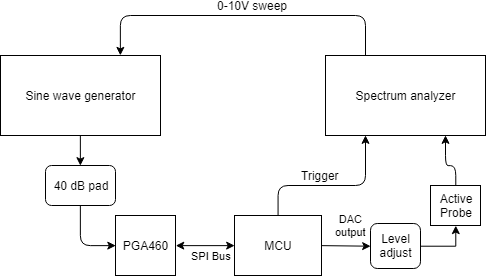
In this test, MCU received a frequency to use from the host PC, configured PGA460 with appropriate BPF coefficients and frequency value, and then continually issued "listen only" command. PGA460 was configured in direct data burst of BPF output, at 8 bit/sample, 65.536 ms record interval, and minimal possible gain of 36 dB. Data was received at 1MSPS by MCU, and converted back to analog via MCU's integrated DAC. This analog signal was fed to a spectrum analyzer. MCU was programmed to generate a pulse for the analyzer upon the first data sample in each "listen only" command, triggering it to do a 110 kHz - 1.1 MHz sweep in 50 ms. A signal generator was synchronized with the analyzer and provided a synchronous sine sweep to the input of PGA460. As a result, in this setup we have received a frequency response plot - which was then retrieved by the host PC.

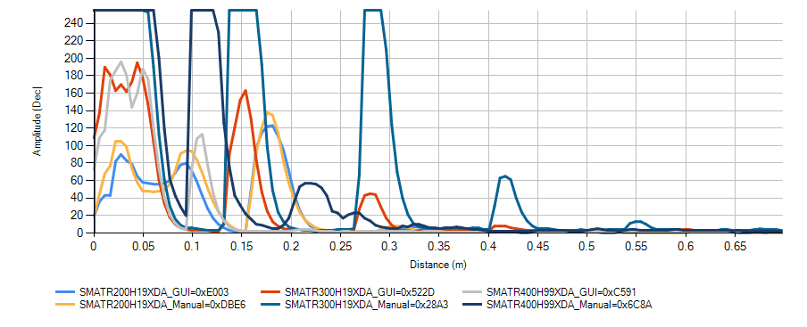
With this setup, we have retrieved a frequency response plot for each configurable frequency in the high frequency mode of PGA460 (180-480 kHz with 1.2 kHz step) which I have attached to this post as a PDF file. Actual peak frequency of the BPF estimated with analyzer's "peak search" function is available in the top right corner below "MKR" label, and the programmed frequency according to the CSV just below that.

PGA460 internal oscillator frequency variation was a concern during measurement. To ensure an acceptable degree of stability during test series (which took around 30 minutes), all equipment, including UUT, were powered up 4 hours before testing started, all testing was performed in temperature-controlled room kept at 30°C, and PGA460's oscillator frequency was measured before and after test run. During both measurements, frequency of 7.968 MHz was observed, with 8 MHz expected. As such, -0.4% frequency offset should be expected. This offset is not corrected for in the plots themselves or the numbers below.

It can be seen that frequency offset indeed exists and is rather significant. At 180 kHz, actual center frequency is around 191k. At 332.4 kHz, it reaches 481.3 kHz, and a step above that the filter completely falls apart and no longer has any discernible response. With the further increase of programmed frequency, it "goes around", and at 362 kHz programmed frequency, it peaks at 115 kHz actual, and continues to rise in frequency after that, however somewhat erratically.

Now, the question: is this behavior expected?

While we could build a lookup table between "actual" frequency and "programmed" frequency and use it to set the filter "properly", it would significantly degrade the resolution of frequency adjustment, especially towards the high frequency end, which is already is not as good as we would like. Our primary frequencies of interest in the high frequency band is 250 kHz, which is well reachable with the current BPF behavior, and 455 kHz, which is not: 453.2 is somewhat low, and 459.8 somewhat high, and they are single step apart - effective resolution of 6.6 kHz. ive 

plots.pdf

  • Hi Sergey,

    I will need a moment to review this data set and confirm the behavior on our bench setup. The roll-over at 362kHz is unexpected.

    In the meanwhile, here is a more detailed explanation on how the digital coefficients are determined:

    The Band-Pass filter works based on digital coefficients B1, A2 and A3. These are calculated based on the burst frequency (FREQ parameter) and Band-Pass bandwidth (BPF_BW parameter). The A2 coefficient is calculated as following:

    • A2= (0.6036*cf^2) +( 2.7401*cf) -32615           ….           For BPF Bandwidth  2kHz.
    • A2= (0.5999*cf^2) + (2.7217*cf) -32415           ….           For BPF Bandwidth  4kHz.
    • A2= (0.5965*cf^2) + (2.6791*cf) -32217           ….           For BPF Bandwidth  6kHz.
    • A2= (0.5928*cf^2) - (2.6726*cf) -32024            ….           For BPF Bandwidth  8kHz.

    Where “cf” is the filter center frequency in kHz (Defined by the FREQ parameter).

    The B1 and A3 coefficients are calculated purely based on the filter band-width:

    • B1=199.7*bw+12
    • A3=-399.3*bw+65512

    Where “bw” is the filter band-width in kHz (Defined by the BPF_BW parameter). Since there will be only four B1 and four A3 coefficients it might be worth to simply store the values instead of doing the calculation. In this case, below are listed the correct values for the B1 and A3 coefficients:

    • B1 = 409 ; A3 = 64718        ….           For BPF Bandwidth 2kHz.
    • B1 = 813 ; A3 = 63909        ….           For BPF Bandwidth 4kHz.
    • B1 = 1213 ; A3 = 63111       ….           For BPF Bandwidth 6kHz.
    • B1 = 1607 ; A3 = 62322      ….           For BPF Bandwidth 8kHz.

    It is important to note that these are scaled-up coefficient values. The true B1, A2 and A3 values are always low number values (typically < +/- 2). The scaling is the following:

    • B1 = B1_real * 2^16
    • A2 = A2_real * 2^14
    • A3 = A3_real * 2^16

    In the digital filter implementation the values are scaled-down right before their use. IMPORTANT: The above coefficient formulas are only applicable for a sample rate of 1us.

  • Hello Akeem,

    As an interim solution, we did our own polynomial fit on the simulated data, made possible by the scaling coefficients you released previously. Coefficients are below:

    Bandwidth

    a

    b

    c

    d

    a3

    b1

    2 kHz

    -1.22935744762526E-12

    9.23946597018039E-07

    -0.027864856528874

    -31746.829190135

    64718

    409

    4 kHz

    -1.21555527164753E-12

    9.12165856196548E-07

    -0.025948693365242

    -31635.7860520422

    63909

    813

    6 kHz

    -1.21129701000412E-12

    9.08469159615466E-07

    -0.026126990017177

    -31392.7054737802

    63111

    1213

    8 kHz

    -1.20585472888359E-12

    9.04117557841391E-07

    -0.026217717891093

    -31163.7630328305

    62322

    1607

    A2 is calculated as a third degree polynomial: a2 = a * fc^3 + b * fc^2 + c * fc + d, with fc - center frequency in hertz (not kilohertz as with TI polynomial).

    We were able to achieve an acceptable fit across the most of the frequency band, however, there are some issues still, for instance, there is significant gain peaking-like behaviour below 100 kHz and above 420 kHz, which manifests as elevated noise floor and, consequently, degraded SNR. While this solution is better than our previous method of tweaking a2 by hand, we would prefer a solution with better behavior on 450 kHz.

  • Hi, Sergey!

    Hi, Akeem!

    I submit the behavior of the chip that Sergey described...

    Sergey! Thanks a lot! For two monthes I can't understand what I'm doing wrong... After reading your post I try to change A2 coeff. and find out that on 250.8 kHz max response is at A2_ti-6900=0xFDDC. (That was measured before you post your fomular. By the way: Your coeff. for that frequency is 0xfffc  and response with it is 2dB less than with 0cfddc. ) I'm planning to use your formular, but i'll try to find why is that difference in responce...

  • We would like to repeat that we are still waiting for TI to respond regarding this issue.

    As I have stated before, we have three frequencies that we are interested in:

    1. 60 kHz. PGA460 meets our requirements at 60 kHz as is.
    2. 250 kHz. Currently we have a stopgap measure implemented, as I've detailed in my previous post. As Kostya correclty notes above, this measure is not perfect. We need to have this issue resolved properly by TI before we go further towards production.
    3. 455 kHz. Performance at 455 kHz does not meet our requirements - or even PGA460 specifications - with or without or modification.

    We would like to see TI either confirm that this is indeed a deviation from the stated specification, and what timeframe is to be expected for a workaround, or confirm that this behavior is intended. We have a tight deadline on this project, and I would like to know whether we need to redesign with a different AFE as soon as practical.

  • Hi Sergey,

    I owe you, Kostya, and other high-frequency users a new GUI and coefficient look-up table. Thanks to your data plots, I was able to spot check and generate a more accurate 3rd order polynomial trend line equation.

    Here is the analysis I performed:

    I spot check the performance of three different Steminc brand high-frequency transducers:

    • SMATR200H19XDA (200kHz)
    • SMATR300H19XDA (300kHz)
    • SMATR400H99XDA (400kHz)

    I swept the entire range of A2 coefficient values currently offered by the 180-480 kHz in the GUI. I then found which A2 coefficient yielded the greatest echo peak amplitude for a fixed distance object detection. Here are the differences between the GUI suggested A2 coefficients versus the manually tuned coefficients for the three transducers:

    Just as you have observed, the lower end (e.g. 200kHz) of the high-frequency range matches more closely between the GUI recommended and the manually optimized A2 coefficient value, while the higher end (e.g. 400kHz) of the high-frequency range shows a much greater mismatch between the GUI recommend and manually optimized A2 coefficient value.

    Using these spot checked data points and your characterization plots of the BPF, I was able to generate new 3rd order polynomial trend line equations for the A2 coefficient. Here is the example for an 8kHz bandpass filter bandwidth: y = -0.0011*x^3 + 0.8241*x^2 - 0.3185*x - 34277

    where:

    • y is the A2 coefficient value in signed 2's order complement integer output
    • x is the transducer center-frequency in kHz

    Here is the charted version of the new A2 coefficient equation (8kHz BPF BW) to show how the actual values compare to the trend line equation based on your BPF plots. The issue with your equation is the roll-over at ~340kHz due to the lack of taking into account the signed nature of the 2's complement value.

    where

      • SPECTRUM refers to your BPF characterization
      • SERGEY refers to your A2 3rd order equation for an 8kHz BPF BW
      • STEMINC refers to the three spot checked transducers

    Here is the tabulated comparison at 10kHz steps:

    Frequency (kHz) A2 Coeff (2'sComp) SPECTRUM A2 Coeff (Hex) SPECTRUM A2 Coeff (2'sComp) EQUATION A2 Coeff (Hex) EQUATION A2 Coeff (2'sComp) SERGEY A2 Coeff (Hex) SERGEY A2 Coeff (2'sComp) STEMINC A2 Coeff (Hex) STEMINC
    180 -14048.69 C920 -4183.709717 EFA9
    190 -12071 D0D9 -12132.405 D09C -1814.710381 F8EA
    200 -10378 D776 -10176.7 D840 597.645028 255 -9242 DBE6
    210 -8446 DF02 -8188.175 E004 3046.121381 BE6
    220 -6576 E650 -6173.43 E7E3 5523.48355 1593
    230 -4253 EF63 -4139.065 EFD5 8022.496406 1F56
    240 -2391 F6A9 -2091.68 F7D5 10535.92482 2927
    250 -438 FE4A -37.875 FFDB 13056.53367 3300
    260 1599 063F 2015.75 7DF 15577.08781 3CD9
    270 3353 0D19 4062.595 FDE 18090.35214 46AA
    280 5887 16FF 6096.06 17D0 20589.0915 506D
    290 7745 1E41 8109.545 1FAD 23066.07079 5A1A
    300 9256 2428 10096.45 2770 25514.05486 63AA 10403 28A3
    310 11559 2D27 12050.175 2F12 27925.80859 6D15
    320 13115 333B 13964.12 368C 30294.09686 7656
    330 15077 3AE5 15831.685 3DD7 32611.68453 7F63
    340 17055 429F 17646.27 44EE 2104.336473 838
    350 18645 48D5 19401.275 4BC9 4298.817564 10CA
    360 20239 4F0F 21090.1 5262 6420.892673 1914
    370 21835 554B 22706.145 58B2 8463.326673 210F
    380 23031 59F7 24242.81 5EB2 10418.88443 28B2
    390 24622 602E 25693.495 645D 12280.33083 2FF8
    400 25812 64D4 27051.6 69AB 14040.43073 36D8 27786 6C8A
    410 26604 67EC 28310.525 6E96 15691.94901 3D4B
    420 27786 6C8A 29463.67 7317 17227.65053 434B
    430 28571 6F9B 30504.435 7728 18640.30018 48D0
    440 29743 742F 31426.22 7AC2 19922.66281 4DD2
    450 30131 75B3 32222.425 7DDE 21067.50331 524B
    460 30906 78BA 32886.45 8076 22067.58655 5633
    470 31292 7A3C 33411.695 8283 22915.67739 5983
    480 31677 7BBD 33791.56 83FF 23604.5407 5C34

    The higher end may require some additional manual fine-tuning, but this equation yields an overall improvement across the entire high-frequency range.

    I will upload the latest version of the GUI and look-up table next early week.

  • Hi Akeem,

    Thank you for the progress report.

    Attached is the worksheet I've used for polynomial fitting. It may be of use to you, as it contains the simulated data: for every defined combination of B2 and A3 and for every possible value of A2 I've done a frequency sweep, analyzed the response, and recorded frequency and amplitude of its peak, if it exists. It is less noisy, more accurate, has more data points, and these data points are distributed evenly across entire range, without compression towards high frequencies displayed in the spectrum analyzer data in my initial post. Do note that A2 values are signed, because I've found that fitting in two's complement directly produces bad fits due to discontinuity around the zero, and all frequencies are in hertz.

    As soon as you have uploaded the new GUI and tables, I'll recheck them on our bench and report back.

    worksheet.xlsx

  • Hi Sergey,

    After implementing my new equation in the GUI, and re-validating the performance of the 200kHz, 300kHz, and 400kHz transducers, I have optimized the GUI based equation for the A2 coefficient as the following: A2_Coeff_at_8kHz = (-0.001*f^3) + (0.658*f^2) + (63.5*f) - 39877

    I have submitted the updated version of the GUI (v.1.0.2.0) for upload to TI.com. It will be available for download this week.

    Here is the updated look-up table:

    Filter No. Freq [kHz] A2_8kHz
    1 180 CD61
    2 181.2 CE55
    3 182.4 CF49
    4 183.6 D03E
    5 184.8 D133
    6 186 D228
    7 187.2 D31D
    8 188.4 D413
    9 189.6 D509
    10 190.8 D600
    11 192 D6F6
    12 193.2 D7ED
    13 194.4 D8E4
    14 195.6 D9DB
    15 196.8 DAD3
    16 198 DBCA
    17 199.2 DCC2
    18 200.4 DDBA
    19 201.6 DEB2
    20 202.8 DFAB
    21 204 E0A3
    22 205.2 E19C
    23 206.4 E294
    24 207.6 E38D
    25 208.8 E486
    26 210 E57F
    27 211.2 E678
    28 212.4 E772
    29 213.6 E86B
    30 214.8 E964
    31 216 EA5D
    32 217.2 EB57
    33 218.4 EC50
    34 219.6 ED4A
    35 220.8 EE43
    36 222 EF3C
    37 223.2 F036
    38 224.4 F12F
    39 225.6 F228
    40 226.8 F321
    41 228 F41B
    42 229.2 F514
    43 230.4 F60D
    44 231.6 F706
    45 232.8 F7FE
    46 234 F8F7
    47 235.2 F9F0
    48 236.4 FAE8
    49 237.6 FBE0
    50 238.8 FCD8
    51 240 FDD0
    52 241.2 FEC8
    53 242.4 FFC0
    54 243.6 B6
    55 244.8 1AD
    56 246 2A4
    57 247.2 39B
    58 248.4 491
    59 249.6 587
    60 250.8 67D
    61 252 773
    62 253.2 869
    63 254.4 95E
    64 255.6 A52
    65 256.8 B47
    66 258 C3B
    67 259.2 D2F
    68 260.4 E22
    69 261.6 F16
    70 262.8 1008
    71 264 10FB
    72 265.2 11ED
    73 266.4 12DE
    74 267.6 13D0
    75 268.8 14C0
    76 270 15B1
    77 271.2 16A1
    78 272.4 1790
    79 273.6 187F
    80 274.8 196E
    81 276 1A5C
    82 277.2 1B49
    83 278.4 1C36
    84 279.6 1D23
    85 280.8 1E0F
    86 282 1EFB
    87 283.2 1FE5
    88 284.4 20D0
    89 285.6 21BA
    90 286.8 22A3
    91 288 238C
    92 289.2 2474
    93 290.4 255B
    94 291.6 2642
    95 292.8 2729
    96 294 280E
    97 295.2 28F3
    98 296.4 29D8
    99 297.6 2ABB
    100 298.8 2B9E
    101 300 2C81
    102 301.2 2D62
    103 302.4 2E43
    104 303.6 2F23
    105 304.8 3003
    106 306 30E1
    107 307.2 31BF
    108 308.4 329D
    109 309.6 3379
    110 310.8 3455
    111 312 3530
    112 313.2 360A
    113 314.4 36E3
    114 315.6 37BB
    115 316.8 3893
    116 318 396A
    117 319.2 3A40
    118 320.4 3B15
    119 321.6 3BE9
    120 322.8 3CBC
    121 324 3D8E
    122 325.2 3E60
    123 326.4 3F31
    124 327.6 4000
    125 328.8 40CF
    126 330 419D
    127 331.2 426A
    128 332.4 4335
    129 333.6 4400
    130 334.8 44CA
    131 336 4593
    132 337.2 465B
    133 338.4 4722
    134 339.6 47E8
    135 340.8 48AC
    136 342 4970
    137 343.2 4A33
    138 344.4 4AF4
    139 345.6 4BB5
    140 346.8 4C74
    141 348 4D33
    142 349.2 4DF0
    143 350.4 4EAC
    144 351.6 4F67
    145 352.8 5021
    146 354 50DA
    147 355.2 5191
    148 356.4 5247
    149 357.6 52FD
    150 358.8 53B1
    151 360 5463
    152 361.2 5515
    153 362.4 55C5
    154 363.6 5674
    155 364.8 5722
    156 366 57CF
    157 367.2 587A
    158 368.4 5924
    159 369.6 59CD
    160 370.8 5A74
    161 372 5B1A
    162 373.2 5BBF
    163 374.4 5C63
    164 375.6 5D05
    165 376.8 5DA6
    166 378 5E45
    167 379.2 5EE3
    168 380.4 5F80
    169 381.6 601B
    170 382.8 60B5
    171 384 614D
    172 385.2 61E5
    173 386.4 627A
    174 387.6 630E
    175 388.8 63A1
    176 390 6432
    177 391.2 64C2
    178 392.4 6550
    179 393.6 65DD
    180 394.8 6669
    181 396 66F2
    182 397.2 677B
    183 398.4 6801
    184 399.6 6886
    185 400.8 690A
    186 402 698C
    187 403.2 6A0D
    188 404.4 6A8B
    189 405.6 6B09
    190 406.8 6B84
    191 408 6BFF
    192 409.2 6C77
    193 410.4 6CEE
    194 411.6 6D63
    195 412.8 6DD6
    196 414 6E48
    197 415.2 6EB8
    198 416.4 6F27
    199 417.6 6F93
    200 418.8 6FFE
    201 420 7068
    202 421.2 70CF
    203 422.4 7135
    204 423.6 7199
    205 424.8 71FB
    206 426 725C
    207 427.2 72BB
    208 428.4 7318
    209 429.6 7373
    210 430.8 73CC
    211 432 7424
    212 433.2 7479
    213 434.4 74CD
    214 435.6 751F
    215 436.8 756F
    216 438 75BD
    217 439.2 7609
    218 440.4 7654
    219 441.6 769C
    220 442.8 76E3
    221 444 7728
    222 445.2 776A
    223 446.4 77AB
    224 447.6 77EA
    225 448.8 7827
    226 450 7862
    227 451.2 789A
    228 452.4 78D1
    229 453.6 7906
    230 454.8 7939
    231 456 796A
    232 457.2 7998
    233 458.4 79C5
    234 459.6 79F0
    235 460.8 7A18
    236 462 7A3F
    237 463.2 7A63
    238 464.4 7A85
    239 465.6 7AA5
    240 466.8 7AC3
    241 468 7ADF
    242 469.2 7AF9
    243 470.4 7B10
    244 471.6 7B26
    245 472.8 7B39
    246 474 7B4A
    247 475.2 7B59
    248 476.4 7B65
    249 477.6 7B70
    250 478.8 7B78
    251 480 7B7E
  • Hi Akeem,

    Your new polynomial works perfectly: we observe a SNR improvement of approximately 3 dB at 250 kHz, and the performance at 450 kHz is now satisfactory.

    Thank you.