

Engineers have struggled for decades to understand the mysterious plot of common-mode voltage (VCM) vs. output voltage (VOUT). The most common VCM vs. VOUT shape appears in Figure 1, although the shape often varies by device and setup configuration.
As VCM approaches the supplies, the input/output limitations of the internal op amps restrict the VOUT range of the device. Therefore, the output swing for an applied VCM often depends on internal op amp topology, supply voltages, gain and reference voltage.

Figure 1. Common-Mode vs. Output Voltage Range of INA114
The test conditions for the datasheet plot in Figure 1 are VS = ±15V and VREF = 0V.
Because many applications require different operating conditions, customized VCM vs. VOUT plots are desirable. An accurate SPICE model and a TINA-TITM test circuit can generate these plots to provide further insight.
Figure 2 shows a TINA-TI test circuit that generates the VCM vs. VOUT plots for the INA114. You can download the simulation file here. If you haven’t installed TINA-TI software, you can do that here.
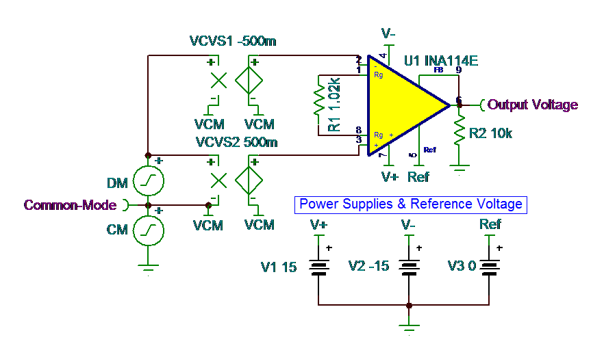
Figure 2. TINA-TI Test Circuit for Generating VCM vs. VOUT Plots
The “CM” source generates a 1Hz common-mode signal with peak-to-peak amplitude equal to the full-range of both power supplies.
The “DM” source and two dependent sources, VCVS1 and VCVS2, generate the differential input signal amplified by the device. I set the amplitude of “DM” at 600mVpp to keep the inputs from greatly exceeding the supply voltages.
To test the output limits of the device, I chose a gain of 50V/V by setting R1 to 1.02kΩ. A 1s transient analysis yielded the plot in Figure 3.
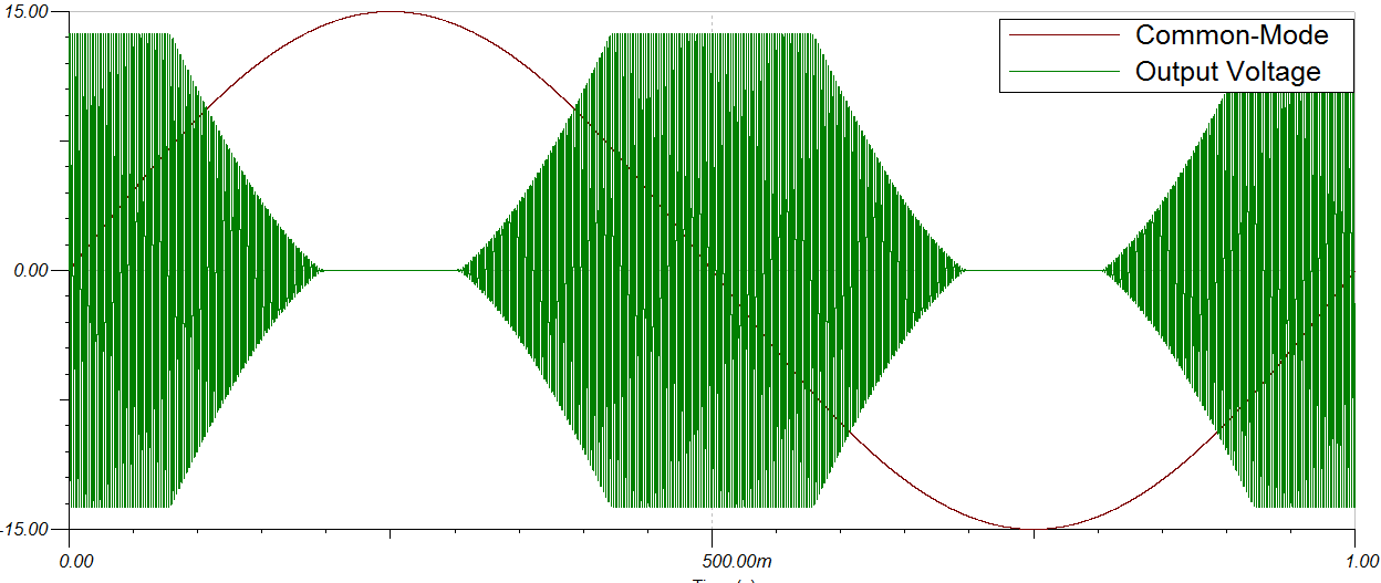
Figure 3. Transient Analysis of VCM and VOUT
Notice that as VCM approaches the supplies, VOUT approaches zero. To get the transient analysis to look more like the datasheet curve, I plotted the output voltage (X) vs. common-mode voltage (Y) using the XY plot feature of the post-processor. The plot in Figure 4 shows that under these test conditions, the simulated plot correlates well with the datasheet curve for the INA114.

Figure 4. INA114 Simulated TINA-TI Plot (Left) and Datasheet Plot (Right)
You can use or modify this TINA-TI test bench to quickly evaluate the accuracy of a SPICE model’s VCM vs. VOUT characteristics, as well as to simulate the effects of changing the operating conditions, as shown in Figure 5.

Figure 5. Simulated VCM vs. VOUT Plot with VREF = 7.5V
So, the next time you find yourself puzzled by an instrumentation amplifier, be sure to consider how the applied operating conditions are affecting the device’s plot of VCM vs. VOUT.

