Because of the Thanksgiving holiday in the U.S., TI E2E™ design support forum responses may be delayed from November 25 through December 2. Thank you for your patience.

This thread has been locked.

If you have a related question, please click the "Ask a related question" button in the top right corner. The newly created question will be automatically linked to this question.

AWR1642BOOST: + DCA1000 EVM ; Calculation of RCS from raw ADC Data ( by using PSD and/or SNR data)

Part Number: AWR1642BOOST
Other Parts Discussed in Thread: AWR1642

Hi, 

1-  This refers to the previous question fro RCS Calculation / Estimation. I have gone through and understood the previous question. I have some additional queries and request guidance of TI team or some other user on the following points. I am deliberately stating the steps that I have carried out. I request you to please go through them, if you find them right, please comment ok and/or extend additional advice if you feel so. If you see them wrong then please advise the right way.

I am using AWR1642BOOST + DCA1000 EVM to capture raw ADC data. I am storing it on a PC and processing it with readDCA1000  MATLAB script provided by TI. This script is producing a matrix of complex values. I am trying to further process this data in MATLAB to have estimate of target Radar Cross Section (RCS).

2-  Please refer page 50 on TI mmwave training pdf file. The screen shot is as follows: 
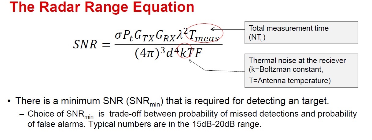
 3-  As indicated int he previous post, I intend to keep all other parameters constant and thus I expect to obtain an estimate of RCS from the SNR values.

4-  In many standard Radar Texts, an additional term "Losses" is included in the denominator of the above equation. However, no such term in included in the above equation. Does TI consider extending advice that should I consider adding the Losses in the above equation to have more realistic and accurate results ? If yes, then what system losses TI could consider advising ? Or, does the equation give a fairly optimal result even without inclusion of losses term ?

5-  I understand that if I use decibel arithmetic for solving the above SNR equation (as commonly and conveniently done in radar calculations) then I must add the antenna gain dB values for transmitter and receiver in SNR equation (addition in dB is analogous to multiplication in linear units). AWR1642BOOST EVM User Guide (swru508b) states peak gain of 10 dB both for the transmitting and receiving antennas. 

Please advise that should I add two antenna gains if I use two transmitters AND should I, for example, add 2 receiver gains if I use two receivers ?

6-  The above equation includes a term lambda (wavelength). We know that wavelength is based on frequency. Suppose that I am using 77 GHz to 81 GHz frequency range for AWR1642BOOST. Please advise which values of frequency should I use for calculating the wavelength ? Will I get optimally good approximate results if I use a single value OR not ? If yes, then in such case should I use 77 GHz, or 81 GHz or 79 GHz (mean of 77 and 81 GHz) ?

7-  The previous post advises : " A convenient way to do this is to have a stationary scenario and use the signal level in the non-zero doppler bins as a measure of the noise floor. "

In an attempt to act on the above advice, I have carried out the following steps:

a)  By using MATLAB, from raw ADC data mentioned in para 1 above,  I extracted a column vector corresponding to a single chirp on a single receiver (a single chirp being used as a prototype step, I will use more chirp later on). I used fft function of MATLAB to obtain the fft of data. I then converted sample index to frequency and I plotted this frequency against Power Spectral Density (PSD). The PSD values are obtained by the formula PSD = abs(rawfft).^2/nfft, which explains that, for each frequency bin/step, I am squaring the magnitude of each complex number and then dividing it by the length of fft.

b)  What do non-zero doppler bins mean / signify in the advice from previous post ? If it is going to be a stationary scenario as advised by TI, then virtually there will NOT be any non-zero doppler bins as there will be virtually no motion observed. I have not taken yet the 2nd fft for doppler estimation, however, I feel that as I have a stationary scenario, I will will have virtually no bin with a doppler level. In such scenario, I feel that the PSD values (after excluding one target peak) could be assumed as noise floor and could be taken as SNR values.

c)  I have a single target case. Therefore, I obtained the PSD value of the single peak corresponding to the target. After that, I took sum of all the PSD values for the whole fft length and then I subtracted PSD value of one dominant peak from that sum. After that, I took average of the remaining (nfft-1) values. 

Now as the PSD value of the target peak has been removed, I assume that the PSD values of remaining (nfft-1) correspond to the noise floor and I take them as SNR. As I mentioned above, I took their average and I am using it as SNR and using it in the above SNR equation. Is my supposition of using PSD as SNR right or not ?

d)  I am then using the above equation with the above obtained SNR value and calculating the target RCS. Does my procedure seem ok ?

Thanking you in advance and regards.

  • Hi Alper,

    We will have one of our algorithm expert reply to your query. Please give us couple of days.

    Thanks,

    Raghu

  • You may benefit from referring to https://e2e.ti.com/support/sensors/f/1023/t/711935 although it is related to oob demo, not offline compute using ADC data.

  • Hi Raghu,

    Thank you for your response.

    I will wait for reply from you and / or your algorithm expert.

    Regards

  • Hi Piyush,

    Thank you for your guidance to the other post.

    I am going to study it.

    In the meanwhile, I will also wait for your algorithm expert.

    Regards

  • Hi Alpher,

    Our expert has already responded to your query. Please check the link provided in the post above.

    Thanks,

    Raghu

  • Hi Raghu 

    Hi Piyush

    Thank you for your advice and indication towards a relevant thread. I went through the indicated thread and got links to other relevant threads as well. Thanks to your advice, I got replies to some of my queries but I request guidance on some pending points.

    For your and my convenience, I am restating my (modified, where needed) questions. I am also stating my understanding of replies to certain questions and request you to please confirm my understanding.

    1)  Although the somewhat similar thread indicated above by Piyush replies some queries, however, it is based on OOB demo. Although I have used and I may still use TI mmwave Demo Visualizer, however, for following reasons, I am avoiding further use of TI mmwave Demo Visualizer:

    a)  One of the main limitations is the UART speed < 1 Mbps. Another one is non-availability of raw ADC data to the user so that user can neither perform basic nor advanced calculations on the radar chip data. I came across the python based script for getting raw ADC data but it was not much helpful.

    b)  I admit that I do not know packages like java and python etc. The source code of mmwave Estimator is written in java so I could not understand it much. 

    c)  As I am interested in developing my own basic understanding and then algorithms using Matlab, therefore, I invested money in DCA1000 EVM to acquire raw ADC data directly. 

    d)  Due to shortage of time and prioritization, I do not wish to invest time and effort in learning java and other computer languages to learn internal functioning of Demo Visualizer and Estimator.

    e) I wish to base my understanding and subsequent use of TI mmwave radar chips on standard radar texts and principles. In view of all above, I hope that knowledge of internal working of Visualier and Estimator and / or their java scripts is not an assumed prerequisite for use of TI mmwave devices.

    f)  In view of above, I earnestly request TI team to please extend guidance on following remaining questions while basing their guidance on raw ADC data and standard radar and signal processing body of knowledge, they may refer MATLAB features if they like , but again that might be a software specific reply.

    g)  I must mention here I am in no way dis-crediting Visualizer and Estimator tools. They are great tools, I have benefited form them a  lot. I am just requesting a more general approach in response to my queries.

    2)  I had inquired about the losses to be incorporated in the Radar Equation. Thanks to your advice, I understand that I can generate a scenario in Estimator and use the default values of various losses in my calculation *using SNR equation mentioned above) to find an optimally accurate solution to the Radar Equation. 

    3)  I tried but I could not obtain answer to this question so I repeat : 

    I understand that if I use decibel arithmetic for solving the above SNR equation (as commonly and conveniently done in radar calculations) then I must add the antenna gain dB values for transmitter and receiver in SNR equation (addition in dB is analogous to multiplication in linear units). AWR1642BOOST EVM User Guide (swru508b) states peak gain of 10 dB both for the transmitting and receiving antennas. 

    Please advise that should I add two antenna gains if I use two transmitters AND should I, for example, add 2 receiver gains if I use two receivers ?

    4)  I had inquired about which frequency value should I use in the above SNR equation for calculating the wavelength (lambda). I found that this question is amicably answered in this thread by TI : http://e2e.ti.com/support/sensors/f/1023/t/689147

    Just for summary I can write here that the average frequency may be used, for details, other user like me may refer this above link.

    5)  I sifted through many threads for my SNR related questions but I could not find a reply although other aspects of SNR are discussed in some threads. Therefore, I repeat my SNR related questions, with special reference to the raw ADC data output from DCA1000 EVM.

    The previous post advises : " A convenient way to do this is to have a stationary scenario and use the signal level in the non-zero doppler bins as a measure of the noise floor. "

    In an attempt to act on the above advice, I have carried out the following steps:

    a) By using MATLAB, from raw ADC data mentioned in para 1 above, I extracted a column vector corresponding to a single chirp on a single receiver (a single chirp being used as a prototype step, I will use more chirp later on). I used fft function of MATLAB to obtain the fft of data. I then converted sample index to frequency and I plotted this frequency against Power Spectral Density (PSD). The PSD values are obtained by the formula PSD = abs(rawfft).^2/nfft, which explains that, for each frequency bin/step, I am squaring the magnitude of each complex number and then dividing it by the length of fft.

    b) What do non-zero doppler bins mean / signify in the advice from previous post ? If it is going to be a stationary scenario as advised by TI, then virtually there will NOT be any non-zero doppler bins as there will be virtually no motion observed. I have not taken yet the 2nd fft for doppler estimation, however, I feel that as I have a stationary scenario, I will will have virtually no bin with a doppler level. In such scenario, I feel that the PSD values (after excluding one target peak) could be assumed as noise floor and could be taken as SNR values.

    c) I have a single target case. Therefore, I obtained the PSD value of the single peak corresponding to the target. After that, I took sum of all the PSD values for the whole fft length and then I subtracted PSD value of one dominant peak from that sum. After that, I took average of the remaining (nfft-1) values.

    Now as the PSD value of the target peak has been removed, I assume that the PSD values of remaining (nfft-1) correspond to the noise floor and I take them as SNR. As I mentioned above, I took their average and I am using it as SNR and using it in the above SNR equation. Is my supposition of using PSD as SNR right or not ?

    d) I am then using the above equation with the above obtained SNR value and calculating the target RCS. Does my procedure seem ok ?

    6)  The thread referred by Piyush ( https://e2e.ti.com/support/sensors/f/1023/t/711935) states that : " The range index to meters conversion is described in the doxygen documentation of the out of box demo in section "Output infromation sent to host" (subsection is "List of detected objects"). Assumed temperature is also in the code and you can set to your environment where you are doing the measurement. "

    As many versions of of mmwave SDk are available in which certain information has been included or excluded over time, and I could not exactly find range index to meter conversion, therefore, can you please indicate a particular mmwave sdk version and exact location of this information in that doxygen ?

    Thanking you in advance and regards.

  • I may not answer in the order in which you raised the questions but I will attempt to see if I can explain you in a way that it makes sense so that if the basics are more clear, you will be able to extrapolate to what you intend to do. I have to admit though that I am no expert in this so take what I say with a grain of salt. From the materials I have come across so far, the RCS estimation does not look like an exact science. It depends on what is your end goal in terms of accuracy of estimation. I don't know if your are doing this an an academic exercise or it is towards some commercial RCS measuring device, because that would be an unconventional use of our sensors, would be useful if you can share what if your goal in terms of application. I guess if yours is a commercial application, you will probably do a calibration against a known RCS device [such as a corner reflector] to take out most of the non-changing quantities in the estimation equation.

    Below I will quote the relevant estimator arithmetic [mostly same in visualizer also] from https://dev.ti.com/gallery/view/1792614/mmWaveSensingEstimator/ver/1.3.0/app/input.js

    ------------------

    var non_coherent_combining_loss = function(num_virtual_rx) {
    if (num_virtual_rx >= 8) {
    return 3;
    } else if (num_virtual_rx == 4) {
    return 2;
    } else if (num_virtual_rx == 2) {
    return 1;
    } else {
    return 0;
    }
    };

    var combined_factor_in_dB = function(tx_power, tx_gain, rx_gain, non_coherent_combining_loss,
    detection_loss, system_loss, implementation_margin, detection_SNR, noise_figure) {
    return tx_power+tx_gain+rx_gain-non_coherent_combining_loss-
    detection_loss-system_loss-implementation_margin-detection_SNR-noise_figure;
    };

    var combined_factor_linear = function(combined_factor_in_dB) {
    return Math.pow(10, combined_factor_in_dB/10);
    };

    var max_range_for_typical_detectable_object = function(rcs_value, combined_factor_linear,
    lambda, num_virtual_rx, chirp_time, min_num_of_chirp_loops, cube_4pi, kB, ambient_temperature) {
    return Math.sqrt(Math.sqrt((0.001*rcs_value*combined_factor_linear*Math.pow(lambda,2)*num_virtual_rx*chirp_time*min_num_of_chirp_loops)/(0.9*cube_4pi*kB*ambient_temperature*1e12)))
    };

    var min_rcs_detectable_at_max_range = function(maximum_detectable_range, cube_4pi, kB,
    ambient_temperature, combined_factor_linear, lambda, num_virtual_rx, chirp_time, min_num_of_chirp_loops) {
    return (0.9*Math.pow(maximum_detectable_range, 4)*
    cube_4pi*kB*ambient_temperature*1e12)/(0.001*combined_factor_linear*lambda*lambda*num_virtual_rx*chirp_time*min_num_of_chirp_loops);
    };

    -------------------------

    The code syntax above isn't too complicated to make sense of the arithmetic it is displaying, so I hope you will be able to digest it at the raw level despite the syntax.

    I want to point to another thread https://e2e.ti.com/support/sensors/f/1023/p/852046/3163323#3163323 the purpose of which is for you to appreciate why we have the 0.9 factor in the estimator calculation above. Although it may be confusing to see the term Beff as 1/fs [later fc correction] which in the estimator is replaced by the time term described in more detail further below.

    The above equation in the estimator assumes you are doing a TDM-MIMO chirping and your processing is basically our oob processing chain. In this chain, we do 1D (range) FFT + 2D (doppler) FFT and then do sum of log magnitudes across the virtual antennas (numTx * numRx). This sum, which is a matrix of dimension number of range bins x number of doppler bins is then fed to the CFAR detection algorithm, which will detect objects if the SNR exceeds the detection SNR set in the CFAR algorithm, all objects above the detection SNR will be detected, the detection SNR is indirectly representing (along with the variant of the CFAR algorithm used) desired probability of detection (Pd in the literature) and probability of false alarm (Pfa). The purpose of the estimator was, for a given detection SNR setting in CFAR [expressing indirectly user intended Pd and Pfa], to let you find the max range for an object of given RCS [beyond the range the SNR from that object would be just below the detection SNR] or to find the minimum RCS required of an object at a given range to be detectable. My understanding is that what you and others who aspire to measure RCS of an object are basically doing is using the same equation to measure the RCS of an object [that may not necessarily be the minimum RCS at a given range where you are placing the object or at the maximum range detectable for this object's RCS] by measuring the SNR itself so the detection SNR is not a threshold of CFAR but the measurement of the SNR itself. The measurement of SNR can be done from the detection matrix just like how the CFAR is measuring before it compares against the detection SNR. If your experiment is controlled in that your object is stationary and nothing else in the scene is moving at the max velocity, this can be done by seeing the range profile and noise profile in the visualizer display - these are nothing but the detection matrix [along the range dimension] at 0th doppler and max doppler bin. So if your object were static, then the level at the range position of the object in the range profile will be the signal power and the noise power will be simply the [mostly flat looking] level of the noise profile and the subtraction [when display in dB] would give the SNR in dB. The range line at max doppler gives a good approximation of receive noise floor unless something in your scene is moving at near the max velocity when it will get messed up.

    One thing to note in above is that the so called object energy in the range profile at the range bin that you see lighted up corresponding to your object is an aggregation of all energies reflected from all objects located at that range bin, there may be several or just clutter at different angles [in elevation and azimuth] which will all appear concentrated in that single bin. If you want more discrimination, you have to go do the angle processing within its limits of resolution. On the other hand, the windowing in the FFTs may broaden the main lobe to spill the energy from the main object bin to neighboring bins [in range, doppler, angle] so you may need to add some neighbors for a more accurate estimation of signal power that is truly representing your actual (point-like) object.

    Related to your question of what you do when you have multiple Tx/Rx, in the basic radar equation, the time term represents the total integration time which in the case of TDM-MIMO involves all the physical chirps and all the Rx antennas. So this total time is either represented by number of virtual rx [=numTx*numRx] * physical chirp time * number of chirp loops, a chirp loop representing the number of chirps related to a single transmit antenna [the dimension involved in doppler FFT], or equivalently it is numRx (typically 4) * physical chirp time * physical number of chirps. The physical number of chirps = numTx * number of chirp loops. Bottomline is that you are considering the full signal integration time that is involved in your signal processing. In radar texts, some of these terms may be represented as "signal processing gain" - when you do an FFT, you get a gain of 10log10(N) because signal is getting concentrated by this amount while noise is not. The gain in fast time (range dimension) is represented here by the physical chirp time term and similarly, the gain in doppler dimension [10*log10(Num doppler bins)] is represented by the slow time dimension i.e number of chirp loops and the numRx similarly represents the multiple rx channel aggregation, all these are enhancing the SNR. So your measured SNR has already been enhanced by these multiplying terms in the time factor and therefore you can see the RCS calculation divides this (enhanced) measured SNR by the enhancement [to give you an intuitive sense], otherwise it would be grossly overestimated.

    While the range and doppler dimension aggregation is coherent, the summing the magnitudes in the (virtual) antenna (angle) dimension is a non-coherent combining operation and so compared to coherent combining, there is a loss which is accounted by the non-coherent combining loss term, this is an empirical coding from some radar text. You can also have a coherent combining processing chain [with much more computational complexity] in which case you don't need this loss [your gain will be fully the numRx factor, you don't have to discount it] but we don't do coherent processing in oob [you may in Matlab].

    Note also that the antenna gains are directional on most of our EVMs [antenna patterns are published in EVM UGs] so dependent on the angle of placement of the object, you may have to account for gain dependence on angle. An automated measurement would probably store measured antenna pattern in a table and pick the value of the gain based on the measured angle [elevation and azimuth] for the estimation of RCS and may need to make it temp dependent for more accuracy.

    With the above understanding, you will be able to make sense of what to do when you have a different chirping scheme than TDM-MIMO, or if you do calculations in Matlab with some assumptions about your scene. For example if you activate all numTx in the same chirp at the same phase say, then you are doing beamforming with max energy at boresight and there will be nulls depending on the Tx spacing [typically 2*lambda on our EVMs between consecutive Tx-es] so for example if your object is at a null, it may see very poor SNR if it is even detectable in the noise/clutter and your RCS measurement will not make sense. In this simultaneous Tx case, you are not really integrating several physical chirp times (corresponding to same Tx like in TDM, you are integrating along the doppler dimension though) but here you will still see enhancement because your transmit power is higher so you will need to multiply your Gtx (in linear domain) by the simultaneous Tx-es you are activating.

    In your simplistic case where you are using only one chirp i.e you don't have doppler information, your reliance on using non-lighted bins to estimate noise power assumes that you have no physical reflections coming from anywhere in your scene except the range bin where the object is placed, this may only be seen in an idealistic anechoic chamber. Using the doppler dimension processing is a more reliable way to see the receiver noise floor as it eliminates all reflections unless any were moving at the max speed. Some customers have also attempted to measure noise by exploring to activate only the receiver while sending nothing on the transmitter [there are some e2e posts on this but I don't recall if this was doable on our sensors].

    PSD is o.k to use, note you don't need to worry bout scale factors [like Nfft] as SNR is relative so fixed scales will cancel out. As usual, when you calculate magnitude square, you do dB as 10*log10(|.|^2), if you estimate magnitude then you do 20*log10(|.|). Averaging noise levels is o.k but generally you will not need to average, you see a flat noise floor when you look at the noise profile in the visualizer. If you wanted to measure the actual dBm level from the ADC samples using FFT, you would need to worry about scaling.

    Range index to meters is based on oob doxygen of SDK 2.1 release. In SDK 3.x, it will be embedded in the code itself (you can study its doxygen and locate the code) as we give out the point cloud x,y,z in meters directly.

  • Hi Piyush, 

    Thank you very much for the detailed response and for cautioning about some intricate aspects.

    Your above response has almost replied my questions. 

    In addition, the following is added:

    I am doing it as a basic academic exercise for ab initio understanding and demonstration of radar principles. However, even for this academic exercise, I intend to use the calibration features of AWR1642 to have accurate and concise results to the extent possible. I also understand that TI sensors are intended basically for detection and ranging and RCS measurement is not their prime purpose; I am trying to study RCS as an indirect measurement.

    I am NOT going to use Visualizer and/or OOB demo for this part of study and I will base my study on raw ADC data and trying to develop my basic radar processing algorithms myself. 

    You are also right that detection SNR is not a concern for me, so far, and I am more interested in signal / receiver SNR estimation. 

    One last question : You mentioned :Using the doppler dimension processing is a more reliable way to see the receiver noise floor as it eliminates all reflections unless any were moving at the max speed. 

    Can you please elaborate it a bit as to how doppler dimension processing is better for estimating receiver noise floor ? Moreover, what if some target is moving with maximum speed in such case ? What will be the problem then?

    Profound thanks again.

  • Regarding your last questions, I want to first make sure we are on same page in terms of what is the noise we are talking about - this is the noise generated in the receiver electronics, mostly thermal noise. Basically the receiver output is reflections from the scene + receiver noise. Note the noise, being generated in the receiver is independent of anything in the scene [the noise does depend on the sensor temp though]. In order to estimate noise, you must guaranteed to not have any reflections or have reflections that are much lower than the noise floor. When you only do range processing i.e have one chirp only and do range FFT, each range bin represents energy reflected from all objects that are at the radial distance represented by that range bin, and there may be multiple such objects at different angles (in 3 dimensions) along the range position and furthermore they could be at any velocity. So unless you have a scene in which the only reflection is coming from the object of your interest (at the range where it is placed) and rest of the range bins are therefore noise, you will not estimate noise correctly. In an office environment for example, you may get reflections from ground and walls [some may be multi-path and may be constructive] at different ranges and this will tend to overwhelm the noise so you will be lucky if you see a single bin showing no reflections [and just the noise] and you will not be able to find out easily even if one exists [if you want you can see what I am saying in the range profile display of visualizer which is like your single chirp range processing as it is the display of range bins at 0 velocity]. The undesired reflections are called clutter, the clutter degrades with range so at higher ranges, the character of receiver output starts to look more like noise. So the way to measure receiver noise reliably is to eliminate all clutter or measure receiver output when there is no transmission [and hence no reflection] i.e the Tx antennas need to be silent while Rxes are enabled [I don't recall our devices can do this].

    The convenience of doppler processing in this case is that it is easy to ensure that in your experimental scene nothing is moving at max velocity during such measurements, whereas it is much harder to control physical clutter because you have to have a idealistic anechoic chamber for that. When something moves at max velocity, its reflection will appear in the max velocity bin at the range at which the object resides and so you cannot use that for noise estimation. You could still see the noise if you knew the velocity [max or otherwise] at which the object moved and so  you would know which doppler bin it will light up [while others still show noise]. If you were to run visualizer and observe the noise profile in a static scene and if you wave your hand fast enough in front of the sensor, you will see the stable noise floor gets disturbed [goes higher] because your motion causes energy from reflection of your hand to appear in the max velocity bin.

    I understand you are trying to learn from first principles but I encourage you to just run the out of box demo with visualizer if you haven't done it as it runs out of flash on power up and visualizer is easy to launch and the range and noise profiles are easy to see, you can look at it to help your learning without getting deep into how the demo or visualizer is implemented, you may be able to appreciate some of the dynamics mentioned above.

  • Hi Piyush,

    Profound gratitude again for taking time and pain to explain the above details and the dynamics.

    I have already worked with and understood to certain extent by using Demo Visualizer but I will refer it again before attempting my own processing of raw ADC data.

    I will also carry out 2D FFT (doppler processing) of raw data and will try to base if for SNR estimation. 

    I may get back to you , if needed, in same or a separate question.

    Regards