


As electrical engineers, most of us were taught as students to analyze operational amplifiers using ideal properties, like infinite input impedance, zero input current, infinite open loop gain, and so on. However, reliance on this ideal model in the absence of an intuitive understanding of device behavior can lead to missteps, especially when the simulator doesn’t catch it, or the math otherwise checks out. Let’s consider one ideal characteristic in particular: the virtual short between the inputs.
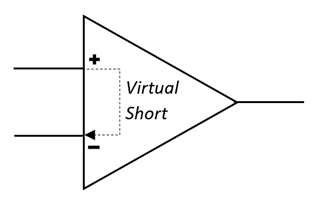
This ‘virtual short’ is a way to describe the amplifier’s tendency to keep the inputs at the same voltage. The actual mechanism for this behavior is that the amplifier examines the difference in the input voltages and adjusts its output until the difference between the inputs is zero. This ability is dependent on the presence of feedback, and the amount that the output has to change in order to align the inputs is determined by the feedback ratio, or gain, of the closed loop. Let’s examine this in the context of a real-world circuit.
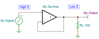
Say, for instance, you need to convert a high impedance signal into a low impedance signal, perhaps to drive sensor voltage measurements down a length of cable with a reasonable amount of capacitance. You don’t want to change the amplitude in this case, you just need a copy of your signal with more drive capability. You might, based on the ideal model, come up with a circuit like this:
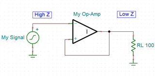
Looks good, right? We have directly connected the output to the unused input, so the amplifier should adjust the output to directly match changes in the input, giving us a feedback ratio of 1:1 and producing a perfect copy of our signal. Ok, let’s do our due diligence and simulate our measurement buffer using an ideal op-amp in SPICE with a 1Vpp 10kHz square wave.
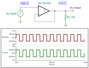
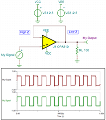
Seems to be working fine with the ideal amplifier, so let’s take it a step further and simulate using our favorite high-speed amplifier, the OPA810.
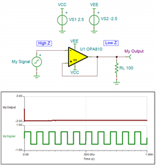
Here we finally start to see the problem with this circuit. The amplifier has railed out to the negative supply, and our measurement data is no longer coming through the buffer. This is a much more accurate representation of the real behavior of this circuit, and if we take a closer look, we can intuitively determine why this makes sense. Notice which input we have placed our signal into, the inverting input of the amplifier. This input will produce an inverted copy of our signal at the output.
Since the output is directly connected to the non-inverting input, this inverted copy is the signal that the amplifier will now compare to the original.
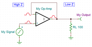
When the amplifier takes the difference of these input voltages, it is subtracting a negative, or adding, which we call positive feedback. As the input signal voltage increases, the output signal decreases, and the amplifier starts to gain up the difference between the two. This creates a runaway condition, and the amplifier rails out to the negative supply. Let’s instead try placing the signal on
the non-inverting input and take another look at our intuitive analysis.
This is looking much better. As the input voltage rises, the output produces the same change. This keeps the inputs aligned and the buffer works as intended. But why didn’t the ideal spice model catch this error? Well, it turns out that the ‘ideal short’ condition that is the source of our mistake exists in the ideal spice model, where the difference between the inputs is assumed to be zero. The inputs are then set to be equal, and the polarity, or sign, of the difference equation is lost. Take a look at this excerpt from the SPICE simulator resources documentation for this topic:
Ideal Operational Amplifiers (Ideal op-amps)-TINA and TINACloud
Analysis Method
We analyze circuits using the two important ideal op-amp properties:
- The voltage between v+ and v– is zero, or v+ = v–.
- The current into both the v+ and v– terminal is zero.
These simple observations lead to a procedure for analyzing any ideal op-amp circuit as follows:
- Write the Kirchhoff current law node equation at the non-inverting terminal, v+.
- Write the Kirchhoff current law node equation at the inverting terminal, v–.
- Set v+ = v– and solve for the desired closed-loop gains.
In the same section you’ll also find that the mathematical derivation of this simplification is based on the “implication of the open-loop gain being infinite,” or the limit as G approaches infinity. Setting the inputs to be equal not only simplifies the mathematical model, it also alleviates some issues that can arise when you ask a numerical tool to deal with zero and infinity.
Non-ideal models, however, need to account for non-ideal phenomena like input offset error and finite loop gain, so they don’t have the luxury of this simplification. This is why the real device simulation caught our positive feedback condition. Let’s now check our corrected buffer circuit that we based on our intuitive understanding and see if it holds up.
Now we can be much more confident that our unity gain buffer will work. We have also gained a better intuitive understanding of op-amp behavior and a healthy appreciation for the limitations of simulation tools.
By: Samuel Burnett