Part Number: JFE150
Other Parts Discussed in Thread: OPA202,
Tool/software:
I'm studying slpa018 application note, I have some questions about article,
Question 1:H
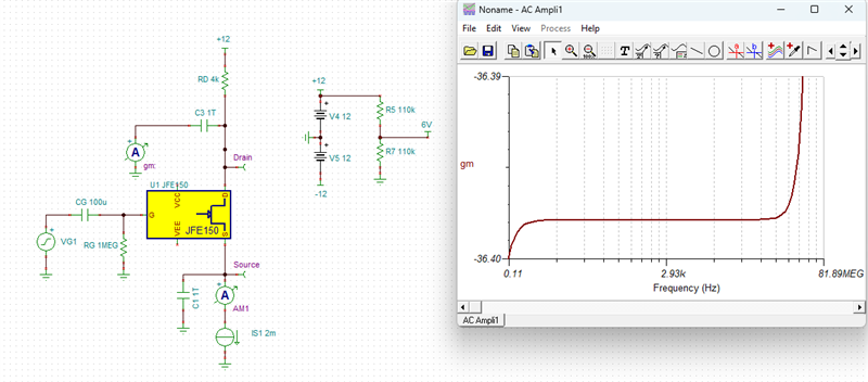
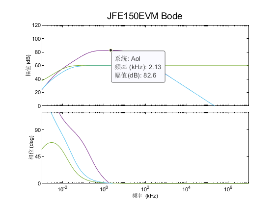
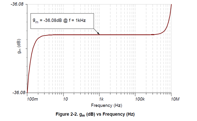
gm vs frequency curve above seems like a simulation result of TINA, isn't ture? If it is, how to simulate gm like this in TINA? As I konw, gm curve is argument of FETwhich is simulated in Virtuoso or else etc.
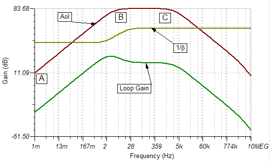
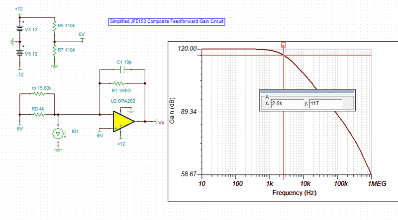
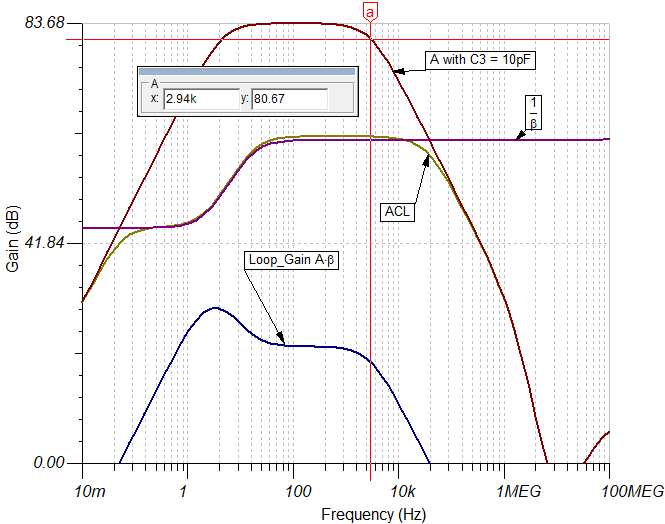
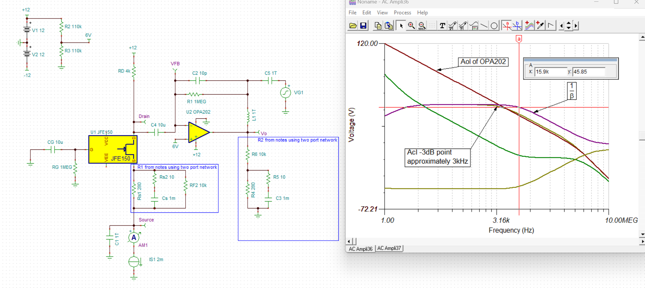
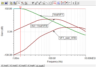
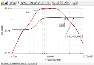
Figure 2-5. Loop Parameters (dB) vs Frequency (Hz)
Question 2:
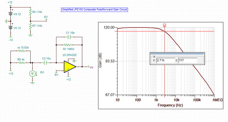
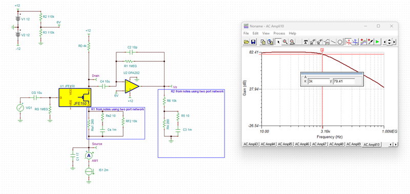
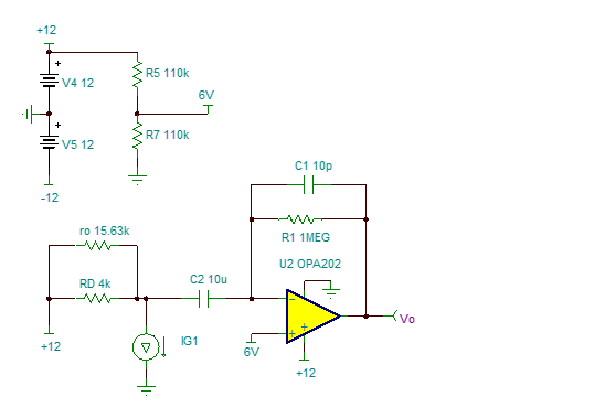
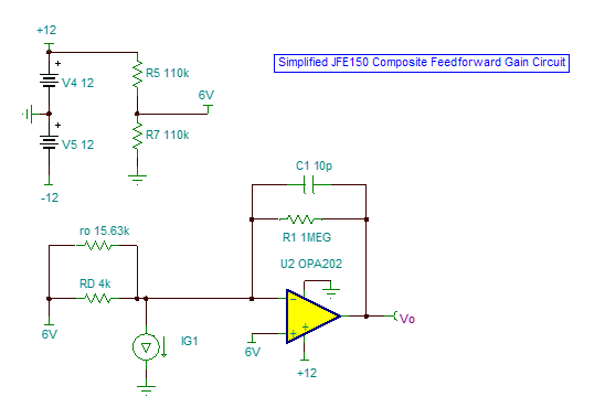
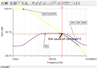
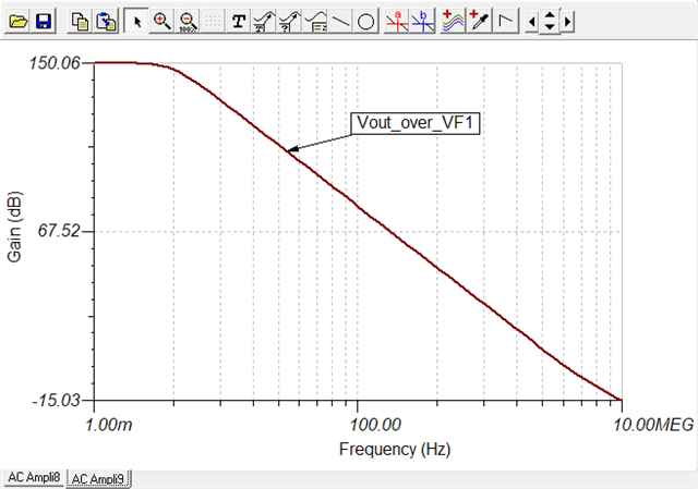
Why there is a 20dB/Dec from A to B? possibly because from A to B in frequency, RD and CD form a high pass filter. Capacitor CD can be viewed as a resistor whose value is larger than RD, ids flow into RD mostly to generate a voltage (of course it’s small signal), and impedance of CD decrease as frequency increase, which make OPA202 inverting amplifier configuration. At frequency above B, CD is shorted compared to RD, so RD is grounded and make no influence, ids flow through R1 to produce output of OPA202. Is it true?
But why there is a -20dB/Dec from C? I think maybe R1 and C1 interact a pole, but 1/(2*pi*R1*C1) is about 16kHz, in fact point C frequency is 2.95kHz, so I’m confused. How to calculate point C frequency ?