This thread has been locked.

If you have a related question, please click the "Ask a related question" button in the top right corner. The newly created question will be automatically linked to this question.

OPA380 Butter-worth response equations

Other Parts Discussed in Thread: OPA380

Hi, I am working on a design of medium bandwidth medium gain a photo-detector using the OPA380, but I am having difficulty with the frequency response characteristics and hoping someone could help me out.


As I will be adding further filtering stages following the transimpedance amplifier a closed form expression for the circuit is important to me so I can set the poles for the transimpedance stage to 2 of the desired high order Butterworth response poles. The datasheet on page 13 shows equations 4 and 5 that talk about designing a second order response using "in the loop feedback" to generate a second pole (see figure 6c) .  I have worked out what I think is a closed form expression for just this stage as:

    Rf / (s^2*Cf*Rf*Cfilter*Rfilter + s*Cf*(Rf + Rfilter) + 1)

From this equation 5 follows only if:

    Cf*(Rf + Rfilter) = sqrt(2) / w-3dB

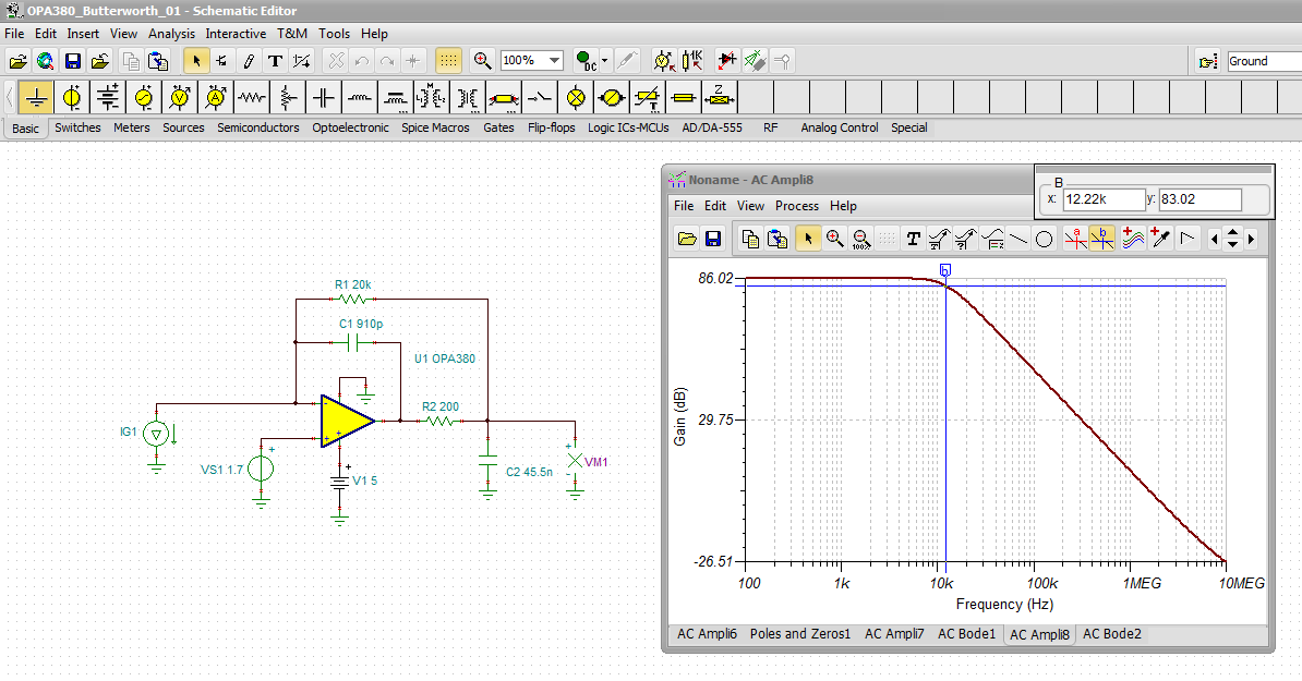
However using the design rule from equation 4 in the datasheet for a Butterworth response I do not see this. For example here is my circuit for a gain of 20,000 and a Butterworth response of bandwidth 12.5KHz supposedly (note I have neglected a model of the photo for simplicity, but since the design equations do no reference any of the photo-diode parameters I am assuming the design equations are independent of these).

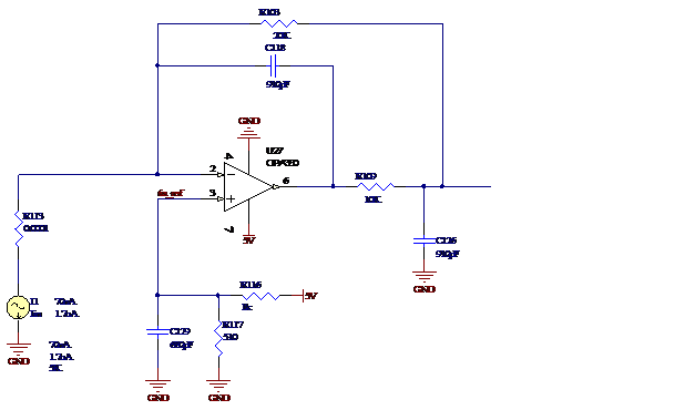
The circuit above satisfies the design equation 4, i.e Cf*Rf = 2*Cfilt*Rfilt.  According to the design equations 4 and 5 in the datasheet this should correspond to a cut-off frequency of f-3dB = 12.4KHz, but based on the transfer function I have calculated above this gives a cut-off frequency of f-6.5dB = 12.4KHz which is 6.5dB down, not the required 3dB for a Butterworth response,  indicating this is not a Butterworth response?


To check my work I also simulated the circuit in spice and plotted my theoretical results over my spice simulation which shows close agreement out to the 1MHz of the simulation.

I want to confirm if my model of the system is indeed accurate? If it is why I am not getting the Butterworth response I expect from the information in the datasheet? If not what is a proper closed form model for this system as I will need to set the poles differently than for a second order Butterworth response?


Thanks

  • Hi Oliver,

    I've been going over the OPA380 second-order Butterworth response issue that you have described. I can't make out the component values shown in your SPICE circuit diagram. Would it possible for you to provide a more clear diagram, or list the values of RF, CF, RFILTER and CFILTER

    Regards, Thomas

    PA - Linear Applications Engineering

  • Thank you Thomas, I can see why you could not make out those values, the copy and paste must have mangled that image quite badly.

    Rf = 20k (ie a gain of 20,000)
    Cf = 910pF
    Rfilter = 10e3 (ie Rf*Cf = 2*Rfilter*Cfilter, equation 4)
    Cfilter = 910pF

    The rest of the circuit is quite simple and I believe should not effect the frequency response. It is a current source on the inverting input to represent an ideal photo-diode (with a resistor of 0.0001 ohms or so, simply so I can measure the input current in the simulation). On the non-inverting pin is a voltage divider to bias the photo-diode at 1.69Vdc (510ohm || 1kohm).

    Thank you.
  • Hello Oliver,

    I spent a lot of time going over the OPA380 Butterworth response problem and did verify your closed-form transfer function is correct. I was able to verify by simulation that the cutoff frequency was around 7.32 kHz, instead of the 12.3 kHz data sheet equation 5 predicted. As I dug deeper I began to find some interesting things about the response of this circuit. 

    With the 10 k RFIL and 910 pF CFIL components you selected the poles created are real poles that lie on the damping axis of the s-plane. This would be the same as occurs with a passive RC low-pass, but in this case two cascaded having different pole frequencies. That does provide a low-pass response, but not a Butterworth response. That makes predicting the - 3dB cutoff frequency not so obvious.

    The OPA380 filter circuit shown in data sheet Figure 6C reminded me of a op amp circuit using an output isolation resistor, plus dual feedback, for stabilization. As I studied the circuit I concluded that although intended for different uses they had much in common. One point about the stabilization method is it emphasized that the output resistor, the same as RFIL, needed to be at least 100x smaller than RF. I believe the reason behind that is to keep the total open-loop output impedance of the op amp circuit low. I then recalculated RFIL and CFIL based on data sheet equation 4, but with RFIL set to 200 Ohms instead of 10 k Ohms. CFIL becomes proportionally larger as expected. 

    When I simulated the OPA380 circuit, the cutoff frequency moved to 12.2 kHz which is almost right on the money. You can see the circuit and response below. Additionally, when I evaluated the pole locations the circuit produces a complex pole pair, which is a characteristic of an active second order response.

    Also, note that the when one reviews the component values in Figure 6C, that RFIL is 100x smaller than RF. This is an important point that isn't mentioned in the text associated with the application. I think if you follow this guideline the OPA380 circuit will provide the performance you are expecting.

    Regards, Thomas

    PA - Linear Applications Engineering


  • Thanks Thomas. This too reminded me of circuits used to stabilise op-amps when driving capacitive loads and I was wondering just last night if the same small Rfilt restriction applied. Looking at my design equations again it shows that as (Rfilt/Rf)^2 approaches 0 the equations approach a Butterworth response which is great

    This means I can now design my poles as needed for the higher order stages using the closed form transfer function above. It might be good to add a note to the datasheet if possible to warn of the restriction of Rfilt << Rf as it is a easy trap to fall into, ie choosing equal capacitance values and designing the resistance.

    Thanks for all your work.
  • One more question on this topic.

    I am now designing with the requirement that Rfilt ~= Rf/10 ... this is leading to quite large values of Cfilt, ie 100nF vs 500pF for Cf using my higher order pole placement ... Will the OPA380 in this configuration, ie with the Rfilt and Cfilt, be OK driving these large capacitances? ... as you mentioned above this circuit looks like one used to stabilise op-amps driving largish capacitive loads so I assume it will do better than the graphs on page 8 of the data-sheet ... I will try in simulation next but I am unsure how well that is modelled in spice

    Thanks.
  • Hi Oliver,

    I am currently traveling and don't have all my resources with me. But as was pointed out the Riso + dual feedback methodology is applied when operational amplifiers are required to drive a large load capacitance. Certainly just using that topology won't assure stability because the the R and C values must be correct to work with the operational amplifier's open-loop gain, phase and complex output impedance.

    The phase margin which is used to verify stability can be determined by circuit simulation. However, doing so requires a simulation model that includes the electrical characteristics I mentioned above. The OPA380 has a good simulation model, but it was developed before we were obsessed with getting the ac characteristics exact. I suspect they aren't spot on in the model and the simulation results may be off some.

    Let me look into this more and especially after I return to the office this coming week. I think we should be able to come to a conclusion about the stability of the proposed circuit.

    Regards, Thomas

    PA - Linear Applications Engineering