This thread has been locked.

If you have a related question, please click the "Ask a related question" button in the top right corner. The newly created question will be automatically linked to this question.

IWR1443: How to calculate range profile in dBFS (or dBm)

Part Number: IWR1443
Other Parts Discussed in Thread: IWR1642

Hello,

My customer is developing their own visualizer tool with running IWR1443/IWR1642 OOB Demo on their target module.
They have already confirmed that works fine, i.e., the same result is being seen in the range profile with your OOB demo visualizer.

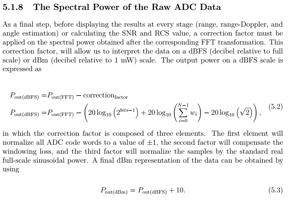
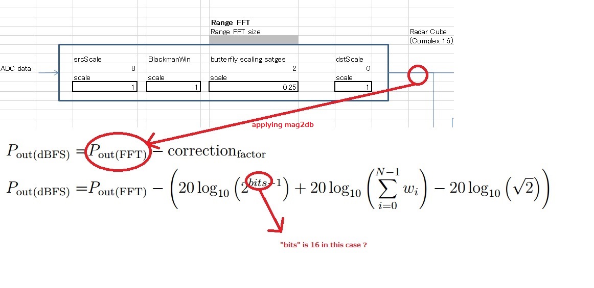
As you know, the range profile on OOB Demo Visualizer indicates the relative power for the detected objects. Now they would like to change the detected power in dBFS or dBm, but don't understand the exact way. 

FYI, here is a snippet from zone occupancy demo MATLAB code (mmwave_industrial_toolbox_<version>\labs\lab0016_zone_occ_14xx\gui\mmw_demo_zone_occupancy.m) to get relative power (rp) :

rp = rp*log2ToLog10*log2Qformat + Params.dspFftScaleCompAll_log;
where, - rp : returned value of Tag;0x00000002 TLV packet - log2ToLog10: 20*log10(2) - dspFftScaleCompAll_log: 1D and 2D FFT related scale value - log2Qformat: depens on the platform. See below if platformType == hex2dec('a1642') log2Qformat = 1/(256*Params.dataPath.numRxAnt*Params.dataPath.numTxAnt); elseif platformType == hex2dec('a1443') || platformType == hex2dec('a1111') if Params.dataPath.numTxAnt == 3 log2Qformat = (4/3)*1/512; else log2Qformat = 1/512; end else fprintf('Unknown platform\n'); return end

This should be the same in OOB Demo Visualizer, right ? They just wanted to know for calculating dBFS(or dBm) for this rp. Could you please suggest ?

Best Regards,
NK


  • Former Member
    0 Former Member

    Hello,

    Please see this response and the thread in general for the suggested approach for determining full scale or relative power to enable determination of dBFS/dBm: 

    https://e2e.ti.com/support/sensors/f/1023/p/821420/3109469#3109469

    Amanda

  • Hi,

    Thanks for your response. I've already read the post you suggested before asking. Unfortunately, it did not answer to our questions.

    Ok, i try to approach from different view point.  I know Pout(dBFS) and Pout(dBm) can be calculated as below. 
    What is the 1st and 2nd element of correct factor in case of OOB demo ? Do you think this can be applied to their use case ?

    Best Regards,
    NK

  • So what is your answer to the above query ?

    Best regards,
    NK

  • Former Member
    0 Former Member in reply to Naoki Kawada

    Hello,

    If you want to use the method described in your literature source you need to be collecting ADC data - this is using the DCA1000. For their use case with the OOB demo the suggested process is as indicated in the previous thread. 

    Amanda

  • Hello, Amanda

    Yes, I know the method i suggested can work in raw data capture environment. In this case, Users can configure data bits and windowing coefficients by their own, so the 1st and 2nd factor can be calculated easily.

    I'm asking what is that value (1st and 2nd factor) in case of OOB demo ? I know 1D fft has been in HWA, so if you can provide the information about HWA FFT windowing spec, i thought we could translate the returned value of OOB demo 1D fft in dBFS(or dBm). Is my understanding correct ?

    You mentioned the answer has been suggested on the following post:

    https://e2e.ti.com/support/sensors/f/1023/p/821420/3109469#3109469

    But unfortunately i could not understand the intention. Could you please pin point the answer ?

    Best Regards,
    NK

  • Refer in the SDK to \ti\datapath\dpc\objectdetection\common\docs\object_detection_data_scaling.xlsx

  • Hello, Piyush_

    Thank you for your answer.

    Please let me confirm if my understanding is correct or not.

    You suggested the scaling applied in HWA looked like this:

    We would be able to get 1D FFT result in radar cube and could convert it to dB form (mag2db). And if we would like to get them in dBFS, did you mean we should additionally take into account about the butterfly scaling in HWA (totally, 0.25) for 1D FFT result (before converting in dB) , and then apply the above calculation ("bits" means 16 in this case)?

    Best Regards,

    NK

  • Former Member
    0 Former Member in reply to Naoki Kawada

    The data format of the 1D FFT can be found from the doxygen: "Range processing only supports 16bits complex data in ImRe format (DPIF_DATAFORMAT_COMPLEX16_IMRE)." at file:///C:/ti/mmwave_sdk_03_03_00_02/packages/ti/datapath/dpu/rangeproc/docs/doxygen/html/index.html

  • bits is 16 as Amanda replied. Yes, you have to take into account the butterfly scaling factor of 0.25. Regarding window scale, I want to clarify that the spread-sheet scaling factors are relative to a pure (Matlab type) implementation, not what you are supposed to use for the window term in the formula e.g the blackman window actually scales [compared to rectangular] by a factor of 2.4 i.e sum(w(i)) for blackman is 1/2.4 times that of sum(w(i)) [= N] for rectangular [you can check in matlab if you like]. So you still have to use the window term in the equation properly. So basically what you have to do in the calculation of the correction term assuming you are using the 1D FFT output of oob implementation is substitute the window term by 20*log10(N/(4*2.4)) [the factor 4 is 1/0.25 the butterfly scaling we are programming in the HWA configuration].

    If you are using the detection matrix output [which is sum log magnitude across virtual antennas of 2D FFT output], then you will have to do a whole bunch of more adjustments based on the spread-sheet information which is more complex calculation. Note that what we display as range profile in the oob plot is not the 1D FFT output, it is the detection matrix output at 0th doppler bin [corresponding to all range bins at 0th doppler] and furthermore we adjust to normalize across different FFT sizes [as I explained the reason in my other post that Amanda quoted and as you can see from the visualizer code you quoted]. And the noise profile plot is from the same detection matrix at the max doppler bin [to give you an the visualization of device's receiver noise assuming your actual scene has no objects moving at max speed, which is typically the case in a stable scene]. Note the range FFT hasn't yet separated the doppler i.e all energy of objects corresponding to different speeds at the same range [in the physical world this would mean they are at different angles] is concentrating in one bin at that range. So whether you use range FFT or doppler FFT output, whether you are picking one bin or a few bins or doing the full energy sum of the FFT bins [which in essence is same as ADC time-domain energy], it depends on what you are trying to accomplish at the high level.

  • Hello, Piyush_

    Thank you very much for your answer. As you suggested, what i would like to do is converting rangeProfile (detection matrix output) from relative power to dBFS form. So I need to have further correction factor in the equation.

    As for the FFT windowing loss, I seem I should care about the scaling compared to rectwin. As you say, in blackman case, it approximately 2.4. And if i talk about hann which is being used for doppler FFT, it would be approximately 2.0. 

    So, I think the FFT windowing loss (20log10(sum(w)) in the equation) corresponds to the sum of the following components:

    • Range FFT part: 20*log10( N / ((1/srcScale)*(sum(RectWin)/sum(Blackman))*(1/butterflyScale)*(1/dstScale)))   
      --> 20*log10(N/(1*2.4*4*1)), where, N=Range FFT size
    • Doppler FFT and log2 output part: 20*log10( N / ((1/srcScale)*(sum(RectWin)/sum(Hann))*(1/butterflyScale)*(1/dstScale)))   
      --> 20*log10(N/(0.0039*2.0*32*1)), where, N=Doppler FFT size

    Is my understanding correct ?

    And how should I care about the correct factor of "SUM Antenna Output - FFT" in the spread sheet ? I think this is not actually FFT. 
    If this is clarified, i think a part of FFT windowing loss in equation is resolved. Because Pout(fft) is in log2 form (detection matrix output), I should convert it to log10 form, and then applying the all of correct factors. 

    Best Regards,
    NK

  • Yes your understanding is correct about the range and doppler FFT terms however note per the xls, the doppler srcscale is dependent on the FFT size (N doppler FFT) itself, please see the color coding on the xls to see what is user input and what is not. So you will realize that butterfly scale factor 0.03125 is 1/N itself and so the doppler FFT factor is simply 20*log10(1/(0.0039*2*1)) [no N dependency, unlike the range term].

    The sum of log2 across virtual antennas is the sum of the log2 magnitude of the individual receive antenna but it is accomplished in HWA using fft and picking the 0th bin (DC) which is simply the sum of the inputs. The scaling is associated with the use of FFT to get the sum in a certain Q format and notice the term "averaging scale" is dependent on the number of virtual antennas, and because FFT is always power of 2, so 12 virtual antennas is summing 16 terms [with zero padding after 12] so the averaging scale is adjusting for this. Note the scalings in this block is relative to Matlab also using FFT to do the sum so the FFT gain factor of Nv (Nv = number of virtual antennas) is there, so while Matlab straight FFT will perform a 12-point FFT and therefore its gain will be 12x, the HWA FFT is doing 16x and hence the averaging scale of 12/16 to adjust. You will need to consider this similar to how you consider the range and doppler FFT scalings [although the name "averaging scale" can be misleading because the FFT output is not trying to average but just sum and in doing this it introduces the N gain]. You have to convert to log10 form and note that it is not 10*log2(.), it is just log2(.), so you have to work out that detail also.

    The dBFs you are trying to get to is not making sense fundamentally for more than one virtual antennas [or ADC channels], but maybe you can establish the equivalence for one antenna somehow from the virtual antenna sum. Note that the powers are added after log2 conversion i.e = sum(log2(|.|)), so in linear the powers are multiplicative (log a + log b = log (ab)), this will complicate things. However, if you assume individual powers are very close to each other (nearly identical) across virtual antennas [an assumption more likely to be satisfied if you do gain/phase compensation], then this term is equal to Nv * log2(|r0|), which may allow you to do the adjustment necessary for dBFs but again, fundamentally speaking what does it mean to say dBFs when you are integrating several receive channels?

    Once you arrive at the correct scalings, it would be good to check if you stream out ADC samples, what you calculate off-line in matlab is matching the adjusted output of the range profile.

  • correction in the first line "doppler srcscale" should be "doppler butterfly scale"

  • Hello Piyush_,

    Sorry for my delayed response.

    Piyush_ said:
    The sum of log2 across virtual antennas is the sum of the log2 magnitude of the individual receive antenna but it is accomplished in HWA using fft and picking the 0th bin (DC) which is simply the sum of the inputs. The scaling is associated with the use of FFT to get the sum in a certain Q format and notice the term "averaging scale" is dependent on the number of virtual antennas, and because FFT is always power of 2, so 12 virtual antennas is summing 16 terms [with zero padding after 12] so the averaging scale is adjusting for this. Note the scalings in this block is relative to Matlab also using FFT to do the sum so the FFT gain factor of Nv (Nv = number of virtual antennas) is there, so while Matlab straight FFT will perform a 12-point FFT and therefore its gain will be 12x, the HWA FFT is doing 16x and hence the averaging scale of 12/16 to adjust. You will need to consider this similar to how you consider the range and doppler FFT scalings [although the name "averaging scale" can be misleading because the FFT output is not trying to average but just sum and in doing this it introduces the N gain]. You have to convert to log10 form and note that it is not 10*log2(.), it is just log2(.), so you have to work out that detail also.

    So, could you please the summarize the above into a single formula (see the text in red) just like the following range and doppler FFT related correction ? I think that would resolve the all of correct factors to get the output in dBFs and then validate it by comparing MATLAB/RawData environment.

    • Range FFT part: 20*log10( N / ((1/srcScale)*(sum(RectWin)/sum(Blackman))*(1/butterflyScale)*(1/dstScale)))   
      --> 20*log10(N/(1*2.4*4*1)), where, N=Range FFT size
    • Doppler FFT and log2 output part :  20*log10(1/(0.0039*2*1))
    • SUM Antenna Outputs FFT part (Log2 output form):
    • Detection Matrix Output Conversion from Log2 to Log10:

    Best Regards,
    NK

  • I believe I have provided sufficient information for you to be able to do the calculations.