This thread has been locked.

If you have a related question, please click the "Ask a related question" button in the top right corner. The newly created question will be automatically linked to this question.

LMP2012: Open loop gain curves

Part Number: LMP2012

Hello,

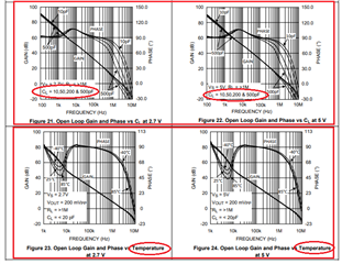
In the LMP2012 datasheet (SNOSA71L –OCTOBER 2004–REVISED SEPTEMBER 2015), there are several open loop gain curves.

Each curve presents the OLG as a function of a special parameter (RL, CL, Vs).

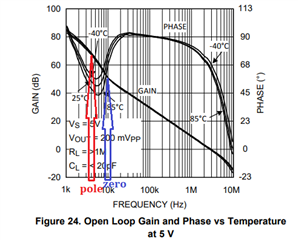
All the curves look very similar except the "figure 23 - open loop gain and phase vs temperature".

I don't understand why there is a big phase dip in that curve ?
Could you explain?

Moreover, I saw Vout = 200mVpp on figure 23.
Is it different for others curves?
Is the testing method different?

Thanks

Simon

  • Hello Simon,

    The LMP2012 curves shown in the datasheet were derived by National Semiconductor before they became part of TI so we don't have any additional information about the original setups beyond what information is provided along with the curves.

    I do see your point about the open-loop gain (Aol) vs temperature curves in Figures 23 (and 24) vs Figures 18 to 22. There is much more of a variation in the open-loop phase at low frequencies in Figures 23 and 24 compared to the others. The Gain, Frequency and Phase scales are more expanded compared to the others, but that doesn't account for most of the differences seen with the phase vs frequency response at low frequencies. Certainly there was some circuit and/or measurement technique differences between these two groups of Aol curves that resulted in the differences.

    Despite the phase differences observed at low frequencies the phase response, and resulting phase margins at high frequencies are comparable among the different graphs and that is the really important aspect of this Aol information. When I look at where the unity-gain cross frequency occurs for all of the graphs it looks like there is at least 30 degrees of phase margin even with a 500 pF load capacitance that only increases outward to 60 degrees with a 10 pF load capacitance. That would indicate that the LMP2012 should be unity-gain stable with the capacitive loads shown in the graphs. 

    Regards, Thomas

    Precision Amplifiers Applications Engineering

  • Hello Thomas,

    I agree with you. We both analyze curves the same way.
    Figures 18 to 22 are used to check the stability at high frequencies.

    Anyway, it seems that in certain conditions there is a phase dip in low frequencies and I would like to know the reason or the method which results in this phenomenon.

    Do you have any idea of the measurement technique used?
    Do you know the meaning of "Vo = 200mVpp" in this context?

    Regard,

    Simon

  • Hi Sim2,

    keep in mind that we are not talking about a standard OPAmp here but a chopping OPAmp. And it's not unusual that the open loop phase versus frequency plot shows some ripple arround the chopping fundamental frequency which is 40kHz here.

    Kai

  • Hi Kai,

    Do you have any reading recommendation about this?

    I'm not familiar with this behaviour.

    Thanks

  • I read the datasheet again following your answer. Something seems weird.

    You say that the chopping frequency appears on the phase curve.
    The phase curve shows a dip at 4kHz; which could indeed correspond to a frequency of chopping.
    On the other hand, figure 5 (Voltage Noise vs Frequency) shows a peak at 40kHz.
    Which is very likely the consequence of chopping.

    But ... 4kHz is not 40kHz ...

    Weird isn't it?

  • Hi Sim2,

    I said arround the chopping fundamental frequency of 40kHz. 4kHz is still arround. 4mHz or 4MHz would not be arround.

    Kai

  • Also, as Thomas already mentioned, crucial for stability is the open loop phase at the unity gain frequency. What happens at much lower frequencies doesn't play an important role.

    There are active filter circuits where the phase margin at low frequencies goes down very much and the circuit is still stable.

    Kai 

  • For me, a decade isn't really around anymore.
    That's why I was asking if there was any literature on the impact of chopping on the phase.

    I agree that stability will be checked at higher frequencies.
    That being said, I find it unsatisfying not to understand the underlying phenomenon. I was hoping you could explain it to me.
    (I did not find anything concrete about the effect on the phase, nor on the protocol showing it.)

  • Simon,

    The dipping in the phase of LMP2012 is clearly caused by the AOL second pole (see red arrow below) and followed by the phase recovery due to a zero (see blue arrow).  And thus the second pole is cancelled by a zero within less than a decade of frequency range resulting in the phase going back to 90 degrees; btw, the first pole is a result of internal Miller compensation stabilizing the circuit and setting overall bandwith of the amplifier.

    Now, without disclosing any proprietary information to the reasons of the second pole followed by cancelling zero, all you need to know is that LMP2012 is actually an auto-zero and not a chopper stabilized op amp (both topologies are called zero-drift).  The difference between the two is that auto-zero amplifier like LMP2012 works by periodically pre-charging a cap with the offset voltage of the amplifier and placing the cap back in series with the input terminal (causing the second pole) to null its offset.  A chopper stabilized amplifier, on the other hand, works by constant switching of the polarity of the input terminals of the first and second stage so the measured offset voltage continually changes its polarity (thus, averaging around zero) while the input signal remains in phase – see diagrams of two different zero-drift topologies below: auto-zero and chopper stabilized amplifier.

  • Hi Marek,
    Thank you for your detailed answer.

    Your analyze about the Figure 24 is very clear.

    In the same way in the Figure 21, I found a zero before the pole. And thus the phase rises up before returning to 90°.
    (The last pole provided by the Cload is obvious.)

    So I come back to my first question. Do you have any idea why phase behaviour is so different between Figure 24 vs 21?
    Maybe the secret is hiden behind the label "Vout = 200mVpp"?
    Is it a nominal behaviour under certain conditions?

    Thanks again for your help.

  • Simon,

    Fig 24 and Fig 21 are quite different because former shows variations due to temperature while the latter variations caused by different capacitive loads - see below - so you compare two vastly different things. Thus, if you want to make such comparison, you need to look at differences between Fig 21 vs Fig 22 or between Fig 23 vs Fig 24 where the only difference is supply voltage.

    Having said that, your question about using 200mVpp signal for any AC analysis may have some merits if this was an input signal, however, in this case the graphs refer only to the output signal - it's likely this was done in gain of 10 or 100.  Also, we have no information what signal amplitude was used in Fig 21 and Fig 22.

  • Hi Simon,

    I made a call yesterday to one of the original National Semiconductor members that was involved in the design and characterization of the operational amplifier products. I asked him what he remembers from the LMP21012 characterization they accomplished. He told me the characterization was done 15 to 20 years ago so his memory about it is limited.

    Here's what we discussed:

    • The open-loop gain (Aol) characterizations were accomplished using the same ATE system for all Figures 18 to 24. The loads and temperature were changed to the conditions indicated in each graph, but otherwise used the same setup. This was a proprietary ATE system developed by National that no longer exists. 
    • The output of the LMP2012 was buffered by another amplifier in the Aol tests. Its input impedance is represented by the RL > 1-Megohm shown on the graphs.
    • All of the Aol test curves seen in datasheet Figures 18 through 24 were taken with VOUT = 200 mVp-p. The input level was adjusted across frequency to maintain the output level of 200 mVp-p. 
    • The issue regarding the more dramatic phase shift at low frequencies seen in Figures 23 and 24 as compared to Figures 18 to 22, may have been caused by the ATE gain/phase analyzer aliasing during the Figure 23 and 24 Aol sweeps. The specific reason for the differences is not known.

    As mentioned previously the actual phase behavior at the low frequency isn't usually a concern, but is at higher frequencies because of the phase margin's effect on stability. You shouldn't have any issues with the LMP2012 AC behaviors - even if the phase margin dips down to 45-degrees between 1 and 10 kHz as Figures 23 and 24 indicate.

    Regards, Thomas

    Precision Amplifiers Applications Engineering

  • Hi Thomas, Hi Marek,

    Thanks for your answers.

    @Marek
    On Figure 21, Vs = 2.7V, CL = 10pF (first case tested) and 50pF (second case), RL = 1M and TA = 25°C.
    On Figure 23, Vs = 2.7V, CL < 20pF, RL = 1M and TA = 25°C (middle case).
    In my opinion, test conditions are the same for at least one curve.

    @Thomas
    Thanks a lot for your call!
    As I understand your last point, the dramatic phase shift isn't a LMP2012 behaviour.

    A little part of mystery remains ;)
    Thanks for your help.