Part Number: AWR1843AOPEVM
A common question is "how should the AWR1843AOP EVM" be positioned and what are the x,y,z axis.
Following snapshot provides this information
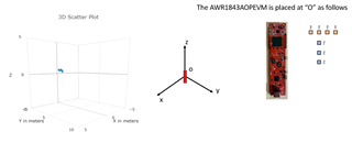
So for example, when the AWR1843AOPEVM is mounted in this position an object detect on the right side of the EVM will have an X>0. If the object is above the board, Z>0
Part Number: DRV5055
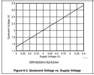
Linear Hall-Effect sensors such as DRV5055 are are often referred to Ratiometric sensors. These devices offer a useful advantage in that the output of the device will scales proportionately with Vcc. For a control system monitoring the output voltage of a sensor, it must do so against a known reference voltage.
Consider the scenario shown below:

Let us suppose first that the Hall-Effect Sensor shown here has a wide Vcc voltage range with a fixed output range of 2V regardless of the Vcc voltage. In this case, Vref for the ADC would ideally be set as close to the maximum output voltage of the Hall-effect sensor to provide the greatest resolution. Due to process, temperature, and voltage related variations, this reference voltage may be difficult to target. Instead, it would be easier to use a fixed reference already present in the system. Vcc makes a easy candidate as it is readily available and known to be greater than the output voltage of the sensor.

The challenge here is that Vcc is often not an ideal fixed voltage. A new error will be introduced whenever there is supply noise or as charge is depleted in battery powered systems. Even if the Hall-effect sensor is continuously operating within an acceptable supply voltage and a static input field, whenever the reference voltage of the ADC shifts, then the final resulting conversion output code will change. To the microcontroller reading the output of the ADC, code changes indicate that the magnet used with this sensor has changed position. Erroneous changes to the position data in a control system represent a significant safety and reliability concern.
Instead, a ratiometric Hall-effect sensor will adjust the output range of the device with respect to the incoming Vcc voltage. In this type of device, the ratio of the output to the Vcc supply remains constant with a fixed magnetic field. Please note the following plots captured from the DRV5055 datasheet.
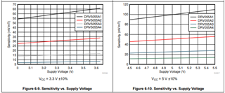
The benefit here is that regardless of supply noise or battery droop, the ADC should receive an input that has a constant ratio respective to the Vcc reference voltage. The Linear magnetic sensing range (BL) is therefore a constant value that represents the maximum input field for any supply voltage that will result in a linear output response for the sensor. As long as the designer keeps the incoming magnetic flux density below BL, the system will provide consistent position information. Additionally, the full scale output range of the sensor will track the full scale input range of the ADC. This will maintain the best overall sensing resolution for the system.
Please consider TI's portfolio of ratiometric sensors available at ti.com
Many of the inductive sensing EVMs can utilize the same debugging process to solve an issue where the EVM won't connect to the GUI. This post will talk about the different possibilities and how to resolve them.
This guide applies to inductive sensing EVMs that use the MSP4305528 in their EVM. Generally, these EVMs use the Sensing Solutions GUI. This includes but is not limited to: LDC1000EVM, LDC1314EVM, LDC1614EVM
Part Number: DRV5032
All you need is a magnet and a Hall-effect sensor and you are all set, right? At a high level, this statement is correct. However, if you are looking for precision when measuring position and triggering when the magnet has reached a specific location, some careful design is needed. This design process entails pairing a suitable magnet with a Hall-effect sensor of appropriate sensitivity. This pairing will depend on several magnet specifications as well as device specifications, which are used in field strength equations. If you are just getting familiar with these equations, you might feel a bit overwhelmed due to the many variables involved. Fortunately, TI has a developed an Excel based tool that already has these equations in place that can quickly get you up to speed with your design.
Magnetic Sensing Proximity Tool
The Magnetic Sensing Proximity Tool allows you to specify magnet specifications including shape, dimensions, and composition. It then allows you to specify how the magnet moves toward your sensor and the range of motion. Lastly it allows you to filter through TI's diverse portfolio of Hall-effect sensors to see which device has the most appropriate sensing capability for the magnet you are using and the movement you want to detect.
Can anyone comment on whether I can use LDC inductive technology for implementing touch buttons on a non-conductive surface?
Which device can be recommended ?
Part Number: AWR6843ISK
I know, this is probably an easy one, but I can't seem to find the answer.
I've looked over many App Notes, User Guides, and Reference Manuals, but I can't seem to find a definition for ISK, in the context of "AWR6843ISK".
The closest I have found was a mention in https://www.ti.com/lit/ug/swru546d/swru546d.pdf in section 1.2 where they reference an "Intelligent Edge Sensor", but I may be wrong.
Is it "Intelligent edge-Sensor Kit?
Fluid sensing is useful in many different medical applications, such as infusion pumps and CPAP machines, where monitoring a dispensing fluid or liquid level is crucial to not only the system’s operation but also to a patient’s health. There are various position sensing technologies available like Hall-effect magnetic sensors and specialty sensors for fluid sensing, and selection of the right sensing technology depends on the specific use case and what degree of accuracy is needed when determining the volume of the liquid. There are numerous applications outside the medical field that need to detect the volume of fluid in a system as well, but this article will focus on medical applications in particular.
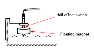
For applications where you only need to detect if the liquid level is high or low (to indicate if a container is full or empty, for instance), a Hall-effect switch with a floating magnet is a cost-effective and simple solution. When the magnet is at a distance outside of the Hall-effect switch’s predefined release threshold (BRP), the sensor will not detect the presence of the magnetic field, indicating that it is in the “off” state. The sensor will switch states to “on” when the magnet is brought closer to the sensor so that it crosses the sensor’s magnetic operating threshold (BOP). Other floating magnet configurations are also possible, such as attaching the magnet to a hinge that is connected to the container wall. Implementation of such a system is a relatively simple mechanical design process, and benefits from a contactless measurement solution that works with high reliability for any type of fluid or container.
The change of state of the Hall-effect switch could send a signal to your system to stop operation until the user refills the liquid or corrective action is taken. This implementation would be useful in applications with a liquid reservoir, such as a CPAP machine, to determine if there is enough water in the tank to create humidity. This solution does not only apply to medical applications and can be applied to any system that cannot operate properly if there is not enough liquid present. TI has a portfolio of Hall-effect switches that are offered in various options such as low/high supply voltage, different packages (SOT-23, X2SON, etc.) and unipolar/omnipolar to fit your system’s requirements. For an introduction to Hall-effect sensors, watch our TI Precision Labs series.
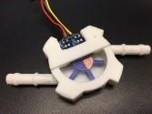
Some applications need to measure the throughput of a liquid through a channel such as a tube. Hall-effect latches are typically paired with ring magnets and can be used to measure the speed and direction of a motor in a liquid pump or flow meter. The alternating north and south poles on the ring magnet toggle the output of the Hall-effect latch which can be used to calculate the speed and direction of the flow meter or pump and from there the amount of liquid flowing can be found. This method of liquid measurement is useful for medical equipment such as dialysis machines where larger amounts of liquid need to be measured through a specific channel such as a tube. To learn more about rotary encoding check out our article Incremental Rotary Encoders.
For applications where higher accuracy is needed or where the liquid needs to remain sterile, a one-dimensional linear Hall-effect sensor can be beneficial. An example of this type of application would be a medical device such as an insulin pump where there is a mechanism similar to a syringe of liquid with a plunger that dispenses the liquid within the equipment. A magnet could be placed on the back of the plunger and as it approaches the linear Hall-effect sensor that is attached to the opposite end of the syringe, you can calculate how much liquid has been dispensed. This solution is contactless, meaning the magnet and sensor would not need to have contact with the liquid in order to determine the liquid level. The DRV5056 is offered in multiple versions, making this device ideal for head-on displacement applications. The different sensitivity variants enable support for various distance and magnet combinations in linear position applications.
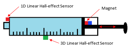
A linear 3D Hall-effect sensor could also be used in applications where a higher degree of accuracy or different positioning of the sensor is needed. By placing the linear 3D sensor on the side of the syringe mechanism as shown above, the magnet will slide by the sensor and give an accurate output by using measurements from the X, Y and Z axes to determine the exact location of the plunger. A multi axis linear sensor, such as the TMAG5170, is beneficial in situations where head on displacement is not possible and more flexibility is required in the placement of the sensor or where the one-dimensional option does not offer enough precision.
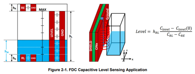
The last solution we will discuss in this article is capacitive liquid level sensing using the FDC1004. Capacitive level sensing is also contactless and can be used to accurately measure liquid height with a resolution as high as <1 mm. This device features active shielding to decrease interference from the outer environment and a flexible system design where the target can be any metal or conductor which is useful for low cost system design. In the diagram below, the sensors in the diagram on the left can be implemented with a flex PCB to fit round or cylindrical container shapes and allow sensor placement on various surface shapes.
The below technical articles are a great place to learn about the FDC1004 and how to implement it in liquid level sensing of fluids that are not conductive.
There are many different ways to implement for liquid level sensing in medical applications in order to assist in monitoring a patient’s health as well as the system’s operation. Various position sensing technologies are available to use in fluid sensing applications, and selection of the right sensing technology depends on the specific use case and the level of precision needed when determining the volume of the liquid. TI has a wide variety of specialty sensors and Hall-effect magnetic sensors to fit your system’s requirements.
This FAQ was written to answer a common request: Computing the Max Range, Range Resolution, Max Velocity, Velocity Resolution for a mmWave Chirp Configuration.
This FAQ provides the theoretical equations and shows how to compute them in an example
Following are the equations to compute these parameters. For more information on the derivation of these equations the reader is invited to review this training
https://training.ti.com/intro-mmwave-sensing-fmcw-radars-module-1-range-estimation?cu=1128486
Active frame time AFT = Tc * #Tx * #chirps/Tx (for MIMO configuration)
Example for following chirp configuration
profileCfg 1 77 7 3 39 0 0 50 1 128 3600 0 0 36
chirpCfg 2 2 1 0 0 0 0 1
chirpCfg 3 3 1 0 0 0 0 2
chirpCfg 4 4 1 0 0 0 0 4
frameCfg 0 2 128 0 100 1 0
Following are the computed values:
Rmax = (0.9*3600e3*3e8 m/s)/(2*50 e12 /s) = 9.72m
Rres = Rmax/128 = 0.076m
Lambda (Wavelength) (77Ghz) = (3e8 m/s) / 77e9 /s) = 0.3/77m = 0.003896
Tc = Idle_Time + rampEndTime = (7+39) usec = 46usec
Vres2 = 3.896e-3m/(2x19.584e-3)s = 0.1 m/s
Is there any requirements/HW or Layout Design Guide for using IWR6843aop? Is it necessary a special material for the pcb?
Thank you in advance!
Part Number: TMAG5170
A major benefit of using a Hall-effect sensor in position sense applications is that it eliminates the physical contact needed to determine position in mechanical solutions. This occurs due to the permeation of magnetic flux from a nearby magnet, which can be used by a linear Hall-effect sensor to produce an output that varies with the changing input field. The magnetic field permeates through air, dust and grime, plastics, and other generally non-ferromagnetic materials. As a result, the sensor can be conveniently placed anywhere a measurable magnetic field is present to provide feedback. One particular challenge that is present when using a linear output Hall-effect sensor is that the magnetic flux density is inversely proportional to the square of the distance from the magnet. As a result, this adds some complexity to position calculations as linear steps produce a non-linear change on the output. While this can be calibrated for any particular magnet, one useful configuration is to orient the magnet and sensor in a slide-by configuration. Here, instead of traveling directly towards the sensor, the magnet travels just above the sensor in a linear path.
As an example, consider the arrangement of a one-dimensional sensor, such as DRV5055 shown in Figure 1 with the magnet traveling either direction along the black line which is parallel to the Y axis. In this example, the pictured magnet is about 22 mm thick with a radius of about 3 mm.
FIGURE1 - Slide-By Magnet Orientation
In this configuration, the sensor will only detect the component of the field vector which is directed along the Z-axis. The resulting input to the sensor over the course of travel for this magnet has an interesting behavior. There is a region approximately the same length of the magnet which produces a linear change in field. With this input, it is now simpler to monitor change in position by measuring in the linear input region.

FIGURE2 - Slide-By Input Field
This can also be easily adapted to increase overall stroke length through the addition of multiple sensors. The process involved with this type of design is discussed in greater detail in Linear Hall Effect Sensor Array Design.
The one dimensional case is limited in range by the length of the magnet. Travel outside the linear input region produces uncertainty in position as there are now two positions that map to the same input magnitude. The uncertainty is resolved by using a three dimensional, 3D, sensor instead. With this sensor type an input field shown in Figure 3 can be observed.
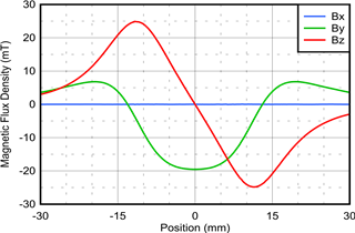
FIGURE3 - 3D Slide-By Input Field
Using this input, three distinct input regions can be defined. The linear region still provides the best correlation for linear motion, but based on the Y component, it is now possible to distinguish the direction approach of the magnet in the non-linear regions as well. Suppose a -6 mT limit is set for By to correspond to the peak values of Bz.
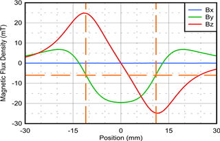
FIGURE4 - Input Field Regions
When By exceeds this threshold the magnet is known to be in the linear sensing region. For By below the threshold, then the sign of Bz will indicate whether the approach is from the right or left. Calibrations can be used to determine the position in this non-linear region, and accuracy will diminish as the magnet moves further from the sensor.
A similar and advantageous approach will again utilize a 3D sensor, but this time the magnet pole will be directed normal to the sensor face rather than parallel. The magnetic field profile across the magnet travel is very similar to the previous example.
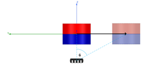
FIGURE5 - Slide-By Mechanical Angle
As the magnet is moved along the Y axis, this motion will produce inputs as shown in Figure 6. In this case, the magnet is much smaller than before with an approximate thickness of 5 mm and a radius of 3 mm. As a result of the orientation change of the magnet, the linear region is now observed on the By component. The width of this region for this particular case is only 6 mm.
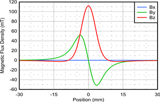
FIGURE6 - Angle Measurement Inputs
Using this data, it is would be possible to use only By to track position, but using the arctangent function will enable position detection over a much wider range.
Electrical Angle: θ = atan 2( Bz , By) 1
Comparing the calculated electrical angle based on the magnetic field inputs to the actual mechanical angle between the magnet and sensor reveals an interesting behavior.
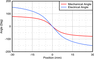
FIGURE7 - Measured Angle vs. Position
While there is a significant error between these two calculations as a result of using magnetic field inputs which do not strictly follow a sinusoidal behavior, it is apparent that the general form of the electrical angle calculation follows the behavior of the mechanical angle. Given this similarity, it should be possible to adjust the electrical calculation to match the actual mechanical angle. When using TMAG5170, it is possible to apply both a gain and offset correction to a single channel which can be represented as α and δ, respectively. Additionally, it is apparent that a second scalar would be beneficial to decrease the overall magnitude. This scalar will be represented by β. This correction would be applied by a microcontroller which is recording the outputs of TMAG5170. Closer analysis also shows that a scaling factor, γ, that increases with angle, can also be helpful in aligning the asymptotic behavior of the two curves at the furthest magnet positions. An example equation based alignment with each of these factors is shown in Equation 2 and Equation 3.
θ′ = atan2 (α × (Bz + δ) , By) 2
θ = β × θ′ − γ × sin θ′ 3
To enable demonstration of this function, please consider the attachment for TMAG5170 EVM shown in Figure 8. Files to enable 3D printing this attachment and physical geometry are available in TMAG5170 Slide-By Attachment.
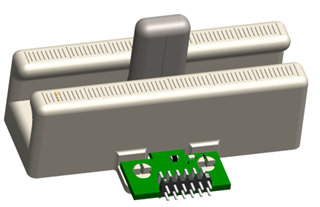
FIGURE8 - TMAG5170 Slide-By Attachment
Based on the simulation data and results of Equation 2 and Equation 3, there are multiple possible implementations with their resulting accuracies. These values and respective errors were determined through inspection. Other methods of linearization, including multipoint calibration, can also prove successful approaches to linearize results. In the following examples three configurations are shown. Configuration 1 applies a scalar correction to the Z axis, and then scales the magnitude of the resulting angle output. Configuration 2, uses these factors as well, but includes an additional intentional offset to help expand the sensitivity range. To help limit error further, configuration 3 adds the final correction factor to help further extend the viewable range of the sensor to the point where input referred noise will likely become the predominant factor for position accuracy.
Table 1. Configurations and Measurement Ranges
|
Configuration |
α | β | δ | γ | Range | Accuracy |
| 1 | 0.6075 | 0.786 | 0 | 0 | +/- 11mm | +/- 0.06mm |
| 2 | 0.6145 | 0.795 | 0.43 | 0 | +/- 21mm | +/- 0.25mm |
| 3 | 0.534 | 0.87 | 0.24 | -7.25 | +/- 23mm | +/- 0.1mm |
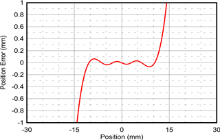
FIGURE9 - Configuration 1
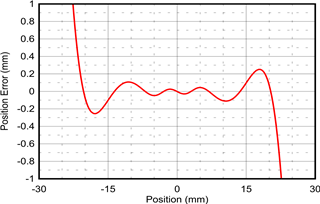
FIGURE10 - Configuration 2
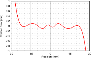
FIGURE11 - Configuration 3
It is also important to remember that these results can vary from system to system as sensitivity error, offset, noise, and mechanical variations will all impact these results which are the theoretical best case behavior. Additional calibration factors can be implemented to improve overall accuracy.
Table 2. Alternative Device Recommendations
| Device | Characteristics | Design Considerations |
| DRV5055 (DRV5055-Q1) | Commercial (Automotive) single axis bipolar linear Halleffect sensor with Analog output available in SOT-23 and TO-92 packages | Analog outputs are subject to electrical noise and calculations require MCU computations. Single axis sensitivity constrains the ability to track movement in free space. |
| DRV5057 (DRV5057-Q1) | Commercial (Automotive) single axis bipolar linear Halleffect sensor with PWM output available in SOT-23 and TO-92 packages | PWM outputs require conversion, but are less susceptible to coupled noise. Single axis sensitivity constrains the ability to track movement in free space. |
| TMAG5170 (TMAG5170-Q1) | Commercial (Automotive) grade linear 3D Hall-effect position sensor with SPI interface available in 8 pin DGK package | Complete magnetic vector sensitivity. This device is able to track a wide range of magnet positions, though careful planning is still required to ensure all input conditions map to a unique position. |
| TMAG5273 | Linear 3D Hall-effect position sensor with I2C interface available in 6 pin SOT-23 package | TMAG5170 has a tighter sensitivity tolerance and TMAG5273 operates over I2C |
Table 3. Related Technical Resources
| Name | Description |
| Linear Hall Effect Sensor Array Design | A guide to designing sensor arrays for tracking motion across long paths |
| Intro to linear Hall effect sensors: Achieve contactless accurate position sensing | A discussion on the differences between a linear output and switched output Hall-effect sensors. |
| What is a Hall-effect sensor? | A discussion about the Hall-effect and how it is used to create magnetic sensors |
| TMAG5170UEVM | GUI and attachments incorporate angle measurement using a precise three dimensional linear Hall-effect sensor |
| TMAG5273EVM | GUI and attachments incorporate angle measurement using a three dimensional linear Hall-effect sensor |
| DRV5055EVM EVM | EVM incorporates a digital display with various sensitivities aligned linearly along a ruler face. |
| TI Precision Labs - Magnetic Sensors | A helpful video series describing the Hall effect and how it is used in various applications |
Source: www.ti.com/.../sbaa513.pdf
